Rigid Body Kinematics

Kinematics or Rigid body kinematics is the study of motion while ignoring the cause of motion. In kinematics, we are interested in “position”, “velocity”, and “acceleration” and the relationship between them. Therefor, in a physical sense, we are interested in describing the motion of \(B\) in \(A\) (see Fig. 4).

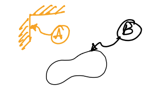
Fig. 4 Motion of a body \(B\) relative to frame \(A\).

Classification of Rigid Body Motion

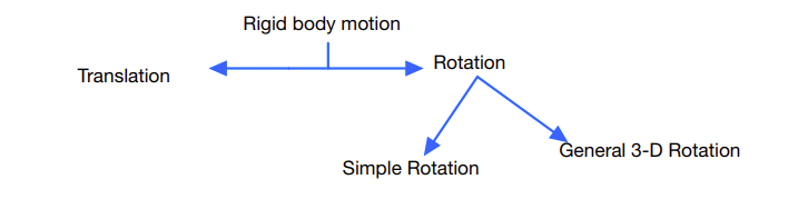
Broadly, there are two classifications for rigid body motion:

• Translation: the motion of \(B\) in \(A\) is a translation if and only if any straight line segment embedded in \(B\) remains parallel to itself when observed from \(A\) when \(B\) moves in \(A\). If this condition is not met, then we have to consider the motion as rotation.

• Simple rotation: the motion of \(B\) in \(A\) is a simple rotation if and only if there exists a unit vector \(\hat{\bf n}\) that remains fixed in both \(B\) and \(A\), as \(B\) moves in \(A\). Examples in figures below:

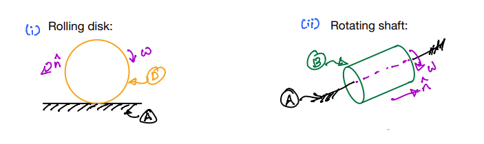
Fig. 5 (i) Disk (D) is in simple rotation with respect to the ground (A). (ii) Shaft (B) is in simple rotation with respect to a fixed axis (A).

Coming back to our old example of a door hinged to a wall.

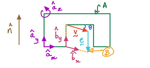
Here, \(\hat{\bf b}_y\) is a unit vector that is fixed in both \(B\) and \(A\). Using our definition for simple rotation tells us that \(\hat{\bf b}_y\) is \(\hat{\bf n}\). So, in mathematical notation, we can say:

(3)\[\hat{\bf n} = \hat{\bf b}_y\]

But we must now pause to ask ourselves if there is any other unit vector that is also fixed in both \(B\) and \(A\)? It turns out that there is, indeed, another one fixed in both \(B\) and \(A\): \(\hat{\bf a}_y\). So, we can now also write:

(4)\[\hat{\bf n} = \hat{\bf a}_y\]

Consequently, from Equations (3) and (4), we get:

(5)\[\hat{\bf b}_y = \hat{\bf a}_y\]

Why is establishing Equation (5) useful and critical?

So far, we have written the vectors \({\bf v}\) and \({\bf e}\), in terms of the \(B\) frame. As a result, they were not functions of \(\theta\).

Expressing the vectors in the unit vectors attached to the A frame requires us to derive relationships between \(\hat{\bf a}_i\) and \(\hat{\bf b}_i\), where \((i = x,y,z)\).

Equation (5) allows us to derive a relationship between \(\hat{\bf a}_i\) and \(\hat{\bf b}_i\), which then provides a basis for developing the rigid body kinematics.

Let us explore how to derive these relationships for the vectors \({\bf e}\) and \({\bf v}\) in the doorwall example (figure is shown again below):

From the second of Equations in (1), we have:

(6)\[{\bf e} = -e\hat{\bf b}_y.\]

Further, by using Equation (5) in Equation (6), we can also see that:

(7)\[{\bf e} = -e\hat{\bf a}_y\]

Terminology

In the preceding example, \(\theta\) is an angle describing the orientation of \(B\) relative to \(A\) (and vice versa). Thus, it is also called an angular position. Other common ways of referring to it are orientation angle or attitude angle.

Now, we come to a more involved example, where we will express \({\bf v}\) in terms of the unit vectors of the \(A\) frame (using the first of the equations (1) as the starting point for this discussion):

(8)\[{\bf v} = v\hat{\bf b}_x\]

We can now examine the relationships between the unit vectors by drawing only the unit vectors with the vector \(\hat{\bf n}\) out of the plane (see figure below this passage).

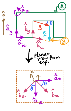
We can then derive the following relationships by examining the lower figure, comprising only unit vectors:

(9)\[\begin{split}\hat{\bf b}_x& = \cos\theta\hat{\bf a}_x + \cos(90 - \theta) \hat{\bf a}_z\\ \hat{\bf b}_z& = \cos(90 + \theta)\hat{\bf a}_x + \cos(\theta) \hat{\bf a}_z,\\\end{split}\]

which can also be written as:

(10)\[\begin{split}\hat{\bf b}_x& = \cos\theta\hat{\bf a}_x + \sin(\theta) \hat{\bf a}_z\\ \hat{\bf b}_z& = -\sin(\theta)\hat{\bf a}_x + \cos(\theta) \hat{\bf a}_z.\\\end{split}\]

Then, from the first of (10):

(11)\[{\bf v} = v(\cos{\theta}\hat{\bf a}_x + \sin{\theta}\hat{\bf a}_z)\]

Along with (5), we have now established the complete relationship between the unit vectors that make up the \(B\) frame in terms of the unit vectors of the \(A\) frame. While this is very useful, we can take these relationships one step further and write the equations in matrix form as follows:

(12)\[\begin{split}\begin{bmatrix} \hat{\bf b}_x\\ \hat{\bf b}_y\\ \hat{\bf b}_z\\ \end{bmatrix} = \begin{bmatrix} \cos{\theta} & 0 & \sin\theta \\ 0 & 1 & 0 \\ -\sin\theta & 0 & \cos\theta \\ \end{bmatrix} \begin{bmatrix} \hat{\bf a}_x\\ \hat{\bf a}_y\\ \hat{\bf a}_z\\ \end{bmatrix}\end{split}\]

Bringing our attention to the second row of the above equation tells us that:

(13)\[\hat{\bf b}_y=\hat{\bf a}_y.\]

Visually, this can be interpreted to mean that the door B swings relative to the wall \(A\) about the \(\hat{\bf b}_y\)-axis, which also coincides with the \(\hat{\bf a}_y\)-axis. In other words, this represents what is known as a simple rotation about the \(y\)-axis. Similar relationships can also be derived for simple rotations about \(x\)-axis or \(z\)-axis.