Table of Contents
Problem 2: Kinetics of System of Particles#
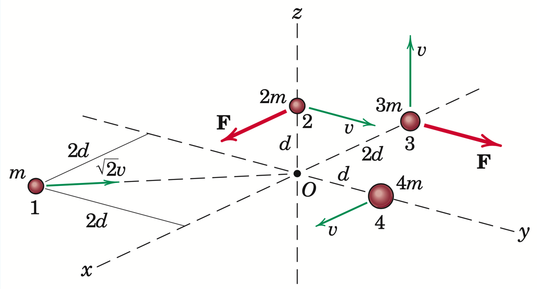
The system of four particles has the indicated masses, positions, velocities, and external forces as shown in the figure above. The inertial frame, \(N\), comprises a set of unit vectors attached to the coordinate system \(x-y-z\) shown in the figure. You have previously calculated the angular momentum of this system of particles about points \(O\) and \(S^*\), the mass centre.
Now, your tasks are to compute:
the velocity and acceleration of the mass centre with respect to the inertial frame \(N\).
the linear momentum of the system of particles.
the time derivative in the inertial frame of the angular momentum of this system of particles about the point \(O\).
the time derivative in the inertial frame of the angular momentum of this system of particles about \(S^*\).
Derivatives must be taken in the inertial frame, N (i.e., using unit vectors attached to the coordinate system shown in the figure).
You may makes use of all the tools you have learned so far in SymPy to complete your work.
Previous Solution Part 1: Angular Momentum of \(S\) about \(O\)#
The theory#
A system of particles \(S\) is provided. You are asked to compute the angular momentum of S about O: \({\bf H}^{S/O}\). In principle, this means computing the angular momentum of each particle and adding them up; this is also known as the composite theorem. This is given by:
\({\bf H}^{S/O} = \sum_{i=1}^4 {\bf H}^{P_i/O}\)
or
\({\bf H}^{S/O} = {\bf H}^{P_1/O} + {\bf H}^{P_2/O} + {\bf H}^{P_3/O} + {\bf H}^{P_4/O}\).
We also have the definition for angular momentum of a generic particle \(P_i\) about \(O\) given by:
\({\bf H}^{P_i/O} \triangleq {\bf r}^{OP_i} \times m_{P_i} ^N{\bf v}^{P_i}\)
, where:
\({\bf r}^{OP_i}\) is the position vector from a point \(O\) to \(P_i\);
\(m_{P_i}\) is the mass of \(P_i\); and
\(^N{\bf v}^{P_i}\) is the velocity of \(P_i\) with respect to a reference frame \(N\).
So, now, we can turn to the features of sympy to compute each of these angular momenta symbolically (as this problem does not assign numerical values to the mass, velocity, or position vectors). Then, we can use the composite theorem to compute the angular momentum of \(S\).
Computing the solution#
from sympy import symbols, sin, cos
from sympy.physics.mechanics import ReferenceFrame, Point, dynamicsymbols
m, d, v = symbols('m d v')
N = ReferenceFrame('N')
---------------------------------------------------------------------------
ModuleNotFoundError                       Traceback (most recent call last)
Cell In[1], line 1
----> 1 from sympy import symbols, sin, cos
      2 from sympy.physics.mechanics import ReferenceFrame, Point, dynamicsymbols
      3 m, d, v = symbols('m d v')

ModuleNotFoundError: No module named 'sympy'
Computing \({\bf H}^{P_1/O}\)#
P1 = Point('P1')
m_P1 = m # mass of P
r_OP1 = 2*d*(N.x - N.y)
P1.set_vel(N, v*(-N.x + N.y))
N_v_P1 = P1.vel(N)
linear_momentum_of_P1 = m_P1*N_v_P1
angular_momentum_of_P1_about_O = r_OP1.cross(linear_momentum_of_P1)
Computing \({\bf H}^{P_2/O}\)#
P2 = Point('P2')
m_P2 = 2*m # mass of P
r_OP2 = d*N.z
P2.set_vel(N, v*N.y)
N_v_P2 = P2.vel(N)
linear_momentum_of_P2 = m_P2*N_v_P2
angular_momentum_of_P2_about_O = r_OP2.cross(linear_momentum_of_P2)
Computing \({\bf H}^{P_3/O}\)#
P3 = Point('P3')
m_P3 = 3*m # mass of P
r_OP3 = -2*d*N.x
P3.set_vel(N, v*N.z)
N_v_P3 = P3.vel(N)
linear_momentum_of_P3 = m_P3*N_v_P3
angular_momentum_of_P3_about_O = r_OP3.cross(linear_momentum_of_P3)
Computing \({\bf H}^{P_4/O}\)#
P4 = Point('P4')
m_P4 = 4*m # mass of P
r_OP4 = +d*N.y
P4.set_vel(N, v*N.x)
N_v_P4 = P4.vel(N)
linear_momentum_of_P4 = m_P4 * N_v_P4
angular_momentum_of_P4_about_O = r_OP4.cross(linear_momentum_of_P4)
Computing \({\bf H}^{S/O}\)#
H_of_S_about_O = angular_momentum_of_P1_about_O + angular_momentum_of_P2_about_O + angular_momentum_of_P3_about_O + angular_momentum_of_P4_about_O
H_of_S_about_O
Previous Solution Part 2: Angular Momentum of \(S\) about \(S^*\)#
The theory#
Here you are asked to compute the angular momentum of S about the system’s mass centre (let’s call it \(S^*\)): \({\bf H}^{S/S^*}\). Once again, this can be done using the composite theorem:
\({\bf H}^{S/S^*} = \sum_{i=1}^4 {\bf H}^{P_i/S^*}\),
where,
\({\bf H}^{P_i/S^*} \triangleq {\bf r}^{S{^*}P_i} \times m_{P_i} ^N{\bf v}^{P_i}\)
But, we haven’t computed \({\bf r}^{S{^*}P_i}\). This requires that we first know the location of the \(S^*\) from \(O\) using the definition of mass centres:
\({\bf r}^{OS^*}= \frac{m_{P_1}{\bf r}^{OP_1} + m_{P_2}{\bf r}^{OP_2} + m_{P_3}{\bf r}^{OP_3} + m_{P_4}{\bf r}^{OP_4}}{m_{P_1} + m_{P_2} + m_{P_3} + m_{P_4}}\).
Then, we can compute \({\bf r}^{S{^*}P_i}\) (which is needed in the computation of each particle’s angular momentum for this section) as:
\({\bf r}^{S{^*}P_i} = {\bf r}^{OP_i}- {\bf r}^{OS^*}\).
Based on this theory, we now complete the computing task as shown below:.
Computing the solution#
r_OSstar = (m_P1*r_OP1 + m_P2*r_OP2 + m_P3*r_OP3 + m_P4*r_OP4)/(m_P1 + m_P2 + m_P3 + m_P4)
r_OSstar
Computing \({\bf H}^{P_1/S^*}\)#
r_SstarP1 = r_OP1 - r_OSstar
angular_momentum_of_P1_about_Sstar = r_SstarP1.cross(linear_momentum_of_P1)
Computing \({\bf H}^{P_2/S^*}\)#
r_SstarP2 = r_OP2 - r_OSstar
angular_momentum_of_P2_about_Sstar = r_SstarP2.cross(linear_momentum_of_P2)
Computing \({\bf H}^{P_3/S^*}\)#
r_SstarP3 = r_OP3 - r_OSstar
angular_momentum_of_P3_about_Sstar = r_SstarP3.cross(linear_momentum_of_P3)
Computing \({\bf H}^{P_4/S^*}\)#
r_SstarP4 = r_OP4 - r_OSstar
angular_momentum_of_P4_about_Sstar = r_SstarP4.cross(linear_momentum_of_P4)
Computing \({\bf H}^{S/S^*}\)#
H_of_S_about_Sstar = angular_momentum_of_P1_about_Sstar + angular_momentum_of_P2_about_Sstar + angular_momentum_of_P3_about_Sstar + angular_momentum_of_P4_about_Sstar
H_of_S_about_Sstar
This solution: Part 1#
We know for a system of particles, \(S\),
\(\frac{^Nd}{dt}{\bf H}^{S/O} = \sum_i {\bf M}^{P_i/O}\),
where \({\bf M}^{P_i/O}\) is the sum of all moments acting on the \(i^{th}\) particle, computed about the fixed point \(O\). There is only one force acting on each particle and the moment is thus trivial to determine as:
\({\bf M}^{P_i/O} = {\bf r}^{OP_i} \times {\bf F}_i\),
where \({\bf F}_i\) is the force on the \(i^{th}\) particle. I compute each particle’s moment below (uch as was done for the previous example of a single particle) with sympy.
# Create magnitude of the force
F = symbols('F')

# For particle 1
F_1 = 0*N.x
M_P1_about_O = r_OP1.cross(F_1)

# For particle 2
F_2 = F*N.x
M_P2_about_O = r_OP2.cross(F_2)

# For particle 3
F_3 = F*N.y
M_P3_about_O = r_OP3.cross(F_3)

# For particle 4
F_4 = 0*N.x
M_P4_about_O = r_OP4.cross(F_4)
This is then equated to \(\frac{^Nd}{dt}{\bf H}^{S/O}\). I store my result in a variable called ddt_H_of_S_about_O, which is the “computing” name for the mathematical expression \(\frac{^Nd}{dt}{\bf H}^{S/O}\).
ddt_H_of_S_about_O = M_P1_about_O + M_P2_about_O + M_P3_about_O + M_P4_about_O#+ other terms that go to zero from lecture 10/11
ddt_H_of_S_about_O
Part 2: about mass centre \(S^*\)#
# For particle 1
M_P1_about_Sstar = r_SstarP1.cross(F_1)

# For particle 2
M_P2_about_Sstar = r_SstarP2.cross(F_2)

# For particle 3
M_P3_about_Sstar = r_SstarP3.cross(F_3)

# For particle 4
M_P4_about_Sstar = r_SstarP4.cross(F_4)
ddt_H_of_S_about_Sstar = M_P1_about_Sstar +M_P2_about_Sstar+M_P3_about_Sstar+M_P4_about_Sstar #+ other terms that go to zero from lecture 10/11
ddt_H_of_S_about_Sstar