JN8: Practice Activity 7

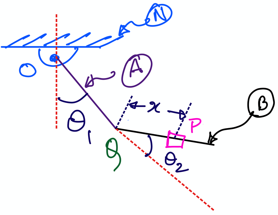
Fig. 12 \(P\) slides on a double pendulum (made up of two links \(A\) and \(B\)).

This notebook use the example of a particle \(P\) sliding on a double pendulum (see figure above); this system was first presented to you in the file “7 Particle Kinematics”. Your objective is to compute the :

1. \(^N{\bf v}^P\), velocity of \(P\) in \(N\); and

2. \(^B{\bf v}^P\), velocity of \(P\) in \(A\).

You are to complete this task using:

1. the defintions of velocity \(^N{\bf v}^P \triangleq \frac{^N d}{dt}{\bf r}_{OP}\) and \(^A{\bf v}^P \triangleq \frac{^A d}{dt}{^N{\bf r}^{QP}}\)

2. the one-point theorem for velocity.

Problem set-up

Create constants using symbols and time-varying scalars using dynamicsymbols

Below we create the scalar constant \(l\), which is the length of the links \(A\) and \(B\); this is stored as the variable l_scalar.:

from sympy import symbols, sin, cos
from sympy.physics.mechanics import dynamicsymbols, ReferenceFrame, init_vprinting
init_vprinting()
l_scalar = symbols('l')

A similar convention for naming variables is used to create theta_1_scalar, theta_2_scalar, and x_scalar to represent \(\theta_1\), \(\theta_2\), and \(x\). These are created as dynamicsymbols as they signifiy the time-varying variables in the figure above. This is done by:

theta_1_scalar, theta_2_scalar, x_scalar = dynamicsymbols('theta_1, theta_2, x')
x_scalar_dot = dynamicsymbols('x', 1)

Create and orient reference frames \(N\), \(A\), and \(B\)

Next, we create the three reference frames \(N\), \(A\), and \(B\), which are stored in the variable names N, A, and B, respectively.

N = ReferenceFrame('N')
A = ReferenceFrame('A')
B = ReferenceFrame('B')

Since we are given the angles between the three reference frames, we can use the .orient method to define the relative orientations using sympy. We can define the between N and A (and also between A and B) using the 'Axis' rotation type within the .orient method, as shown below:

A.orient(N, 'Axis', (theta_1_scalar, N.z))
A.ang_vel_in(N)

B.orient(A, 'Axis', (theta_2_scalar, A.z))
B.ang_vel_in(N)

Create the points \(O\), \(Q\), and \(P\)

Next, we need to create three points:

1. \(O\) is the point of contact between link \(A\) and ceiling \(N\); the corresponding variable name we use is O

2. \(Q\) is the point of contact between link \(A\) and link \(B\); the corresponding variable name we use is Q

3. \(P\) is also modeled as a point (massless particle) that slides on the link \(B\); the corresponding variable name is P.

Each of these points is made using Point, which we import from sympy.physics.mechanics, as below:

from sympy.physics.mechanics import Point
O = Point('O')
Q = Point('Q')
P = Point('P')

You can see that this command is quite similar in its syntax to how we create a reference frame using sympy’s ReferenceFrame feature. As you have seen in this and preceding activities, once we have created a ReferenceFrame, we can exploit methods such as orient, set_ang_vel, and set_ang_acc to describe the orientation kinematics. Similarly, we can use the Point class to define the translational kinematics; in other words, we can exploit methods that are bundled with the Point feature of sympy to:

1. describe position vectors between points using .set_pos;

2. define the velocities of points in different frames using .set_vel; and

3. accelerations of points in different frames using .set_acc.

In the remaining discussion of this chapter, we see how to use these methods in computing the kinematics of points by implementing computational versions of the two-point theorem abd one-point theorem. Let’s get started……

From, the figure, we know that \({\bf r}^{OQ}\) is the position vector from \(O\) to \(Q\). We can use sympy to define the location of \(Q\) using the .set_pos() method on that point. The .set_pos() method requires that you (the user) provide two additional details to it:

1. The point from which \(Q\)’s location is defined relative; in this case, it is \(O\).

2. The component form of the vector in an appropriate reference frame. In this case, \(l \hat{\bf a}_y\) is the position vector \({\bf r}^{OQ}\), so we provide this as l_scalar*A.y to the .set_pos(). This is shown below:

Q.set_pos(O, l_scalar*A.y)

As you can see, this method does not print anything in an output cell. However, the computer stores this information internally. To access this information, we have another method that we can use for any point called .pos_from. This can be used to examine the position vector as shown below. Note that, I choose to actually store the output of .pos_from in a variable name r_OQ_vector as I know I will need it later for my computations of the two-point theorem.

r_OQ_vector = Q.pos_from(O)
r_OQ_vector

Similarlyl, we can configure the \(P\) by making use of the two methods described above, set_pos and pos_from, on P. Then, we can store the position vector information about P relative to Q (i.e., \({\bf r}^{QP}\)) in the variable name r_QP_vector. This is shown below:

P.set_pos(Q, x_scalar*B.y)
r_QP_vector = P.pos_from(Q)
r_QP_vector

Now, from out lecture notes, we know that \({\bf r}^{OP}\),the position vector from \(O\) to \(P\), is given by:

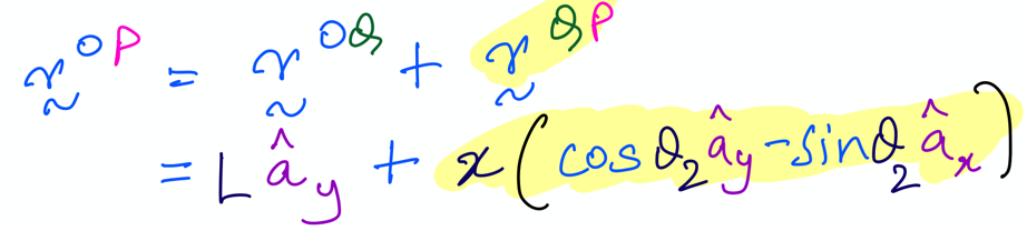
So, we can use sympy and our knowledge of vector addition to compute this position vector using the r_OQ_vector and r_QP_vector. I store this information in a variable r_OP_vector, as shown below:

r_OP_vector = r_OQ_vector + r_QP_vector
r_OP_vector

Next, I describe how we can exploit sympy and our knowledge on vector calculus to compute velocities of \(P\) from diffrerent reference frames.

Approach 1: Using definitions

Compute \(^N{\bf v}^P\)

The classical definition of velocity is well known (see figure below):

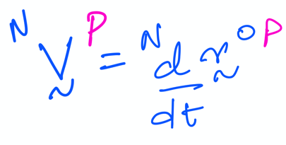
We use that and our knowledge of taking time derivatives in sympy to compute \(^N{\bf v}^P\), which is stored in the variable N_v_P_approach1.

N_v_P_approach1 = r_OP_vector.dt(N)
N_v_P_approach1.express(A)

Compute \(^A{\bf v}^P\)

\(^A{\bf v}^P\) is also computed in a similar fashion using classical definition and sympy; this information is stored in the variable name A_v_P_approach1. See below:

A_v_P_approach1 = r_QP_vector.dt(A)
A_v_P_approach1.express(A)

Approach 2: Implementing one point theorem

In this section, we learn to compute the two velocities \(^N{\bf v}^P\) and \(^A{\bf v}^P\) using the one-point theorem.

Compute \(^N{\bf v}^P\)

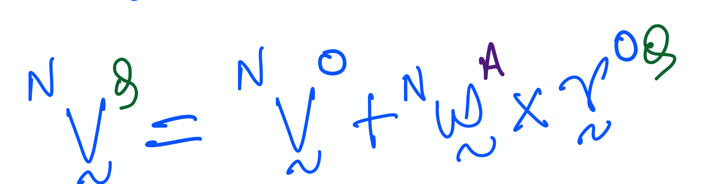
To begin, we must first identify correctly how to utilize the one-point theorem. This has been explained in the video lecture so reference that to referesh your memory. In the image below, the resulting equation from correctly applying the one point theorem to compute \(^N{\bf v}^P\) is repeated from the handwritten notes :

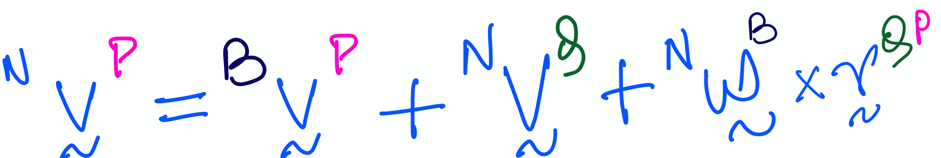
The right hand side of the above equation tells us what we need to compute. Specifically, it tells us we will need to compute the following to determine \(^N{\bf v}^P\) in sympy:

1. \(^B{\bf v}^P\), which we can easily evaluate from the figure;

2. \(^N{\bf v}^Q\), which we compute using the two-point theorem. This is discussed in greater detail below (and also covered in the lecture notes);

3. \(^N{\bf \omega}^B\); this information is actually already available from approach 1 above, where we used the .orient method. However, we haven’t stored this in a variable, which we will do in the steps that follow below; and

4. \({\bf r}^{QP}\), which we have already computed above for Approach 1; this is already stored in the variable name r_QP_vector.

Step 1: Define \(^B{\bf v}^P\) using .set_vel

From the figure, we can easily compute the \(^B{\bf v}^P = \dot x \hat {\bf b}_y\). We can then use the .set_vel to set the velocity of P in the B-frame. This is then stored in the variable B_v_P_vector using .vel method.

_The difference between .set_vel and .vel: the former lets us define the velocity and store it within the computer without an output; the latter method allows a human to access the velocity vector for future computation. In other words, their behaviour is similar to what we see for creating position vectors using .set_pos and accessing it using .pos_from.

This is shown below:

P.set_vel(B, x_scalar_dot*B.y)
B_v_P_vector = P.vel(B)
B_v_P_vector

Step 2: Compute \(^N{\bf v}^Q\)

To compute this velocity, \(^N{\bf v}^Q\), we make use of the two point theorem. This is shown below from the lecture notes:

From the figure it is clear that point \(O\) is fixed in the two frames \(N\) and \(A\). So, for all our sympy-bsed computations, we need to ensure that \(O\) is fixed in frames \(N\) and \(A\) as a point of zero velocity. This is done using our tried and tested .set_vel method, as shown below:

O.set_vel(N, 0)
O.set_vel(A, 0)

Further, as we know that the two-point theorem for \(^N{\bf v}^Q\) requires \(^N{\bf v}^O\), we store this latter velocity in the variable named N_v_O_vector using the .vel method.

N_v_O_vector = O.vel(N)

In approach 1, we defined the orientaion of \(A\) in \(N\). So, we can easily use the .ang_vel_in method to store the angular velocity of A in N (\(^N\omega^A\)) in the variable N_w_A_vector:

N_w_A_vector = A.ang_vel_in(N)

Finally, we can compute the \(^N{\bf v}^Q\) by defining the the two-point formula, as below:

N_v_Q_vector = N_v_O_vector + N_w_A_vector.cross(r_OQ_vector)
N_v_Q_vector

Step 3: Store \(^N\omega^B\) for use in one-point formula

We can store \(^N\omega^B\) in the variable N_w_B_vector using the .ang_vel_in method on B, as shown below:

N_w_B_vector = B.ang_vel_in(N)

Step 4: Finally, compute \(^N{\bf v}^P\)

Now, we can finally compute the \(^N{\bf v}^P\) by implementing the one point theorem (repeating the hand-written equation so you can avoid scrolling up):

Indeed, we will store \(^N{\bf v}^P\) in a variable named N_v_P_vector_approach2 to be clear that we are using our second approach here. In sympy, we implement the handwritten equation to compute \(^N{\bf v}^P\) by making use of vector addition (which you have already learned) as follows:

N_v_P_vector_approach2 = B_v_P_vector + N_v_Q_vector + N_w_B_vector.cross(r_QP_vector)
N_v_P_vector_approach2.express(A)

Compute \(^A{\bf v}^P\)

By one-point theorem, we know that \(^A{\bf v}^P\) can be evaluated using:

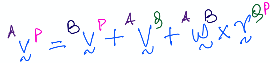
So, we can do this entire computation in sympy through the few lines of code written below (This is very similar to how we computed \(^N{\bf v}^P\)). Note that:

1. we have already computed and stored \(^B{\bf v}^P\) in B_v_P_vector; and

2. we have already computed and stored \({\bf r}^{QP}\) in r_QP_vector.

We discuss the evaluation of the other terms in the below steps.

Step 1: Set velocity of \(Q\) to zero in \(A\) and \(B\)

Since Q is a point shared by and also fixed in the bodies \(A\) and \(B\), we use the .set_vel method to set its velocity to be zero. We then store this in the A_v_Q_vector for accessing in later computations:

Q.set_vel(A, 0)
Q.set_vel(B, 0)
A_v_Q_vector = Q.vel(A)
A_v_Q_vector

Step 2: Store \(^A\omega^B\) to use in one-point theorem

In approach 1, we already used the orient method on \(B\) to define its orientaiton relative to \(A\). So, we can readily access its angular velocity using the .ang_vel_in method on B. For future use, we store \(^A\omega^B\) in the variable A_w_B_vector, as shown below:

A_w_B_vector = B.ang_vel_in(A)

Step 3: Finally, compute \(^N{\bf v}^P\)

Now, we can finally compute the \(^A{\bf v}^P\) by implementing the appropriate version of the one-point theorem in sympy. We store \(^A{\bf v}^P\) in the variable A_v_P_vector_approach2.

A_v_P_vector_approach2 = B_v_P_vector + A_v_Q_vector + A_w_B_vector.cross(r_QP_vector)
A_v_P_vector_approach2.express(A)

We can also compare that the resulting velocities are the same using either approach by comparing the A_v_P_vector_approach2 is identical to A_v_P_vector_approach1 as below:

A_v_P_vector_approach2.express(A) == A_v_P_approach1.express(A)

True

In English, we can say that the above input line is essentially us asking the computer: is the A_v_P_vector_approach2 the same as A_v_P_approach1? Or, in other words, are the two approaches to computing velocities identical?

The == sign is one type of a comparison operator in computer programming. For those interested in learning more, they are discussed here.