JN2: Practice Activity 1

This is an interactive notebook that is a companion to the in-class lectures; specifically this notebook addresses the Practice Activity 1 (PA1).

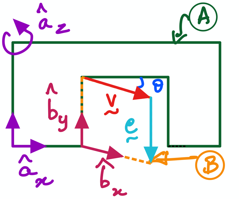
This activity implements the door-wall example (see figure above) as an interactive textbook that works in JupyterLab. The activity is referred to as Practice Activty 1 (PA1) in your handouts used during in-class lectures. Your goal is to implement the two handwritten equations (see Equation 1 below) into the code cells using sympy’s feature set.

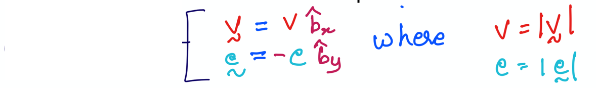
The above handwritten equations can be written in typeface as:

(2)\[\begin{split}{\bf v}& = v \hat{\bf b}_x\\ {\bf e}& = -e \hat{\bf b}_y\end{split}\]

where \(v\) and \(e\) are the magnitudes of \({\bf v}\) and \({\bf e}\).

Create scalars using “symbols”

from sympy import symbols

We begin by using sympy’s symbols to create the scalars \(v\), \(e\) and \(\theta\), as shown below:

v, theta, e = symbols('v theta e') # These are scalar symbols.

v

\[\displaystyle v\]

theta

\[\displaystyle \theta\]

e

\[\displaystyle e\]

Creating Reference Frames

A and B are reference frames that make up the wall and the door, respectively. Let’s create them. First, we need to gain access to the ReferenceFrame feature that is provided to us by sympy.physics.mechanics in the following way:

from sympy.physics.mechanics import ReferenceFrame

Then, we have to specifically create the wall A’s reference frame to gain access to the set of 3 dextral unit vectors \({\hat {\bf a}_x}\), \({\hat {\bf a}_y}\), and \({\hat {\bf a}_z}\) as below:

A = ReferenceFrame('A') # This creates the unit vectors that make up the wall's frame A

The reference frame attahed to the door B can also be created in a similar fashion so that we gain access to the set of 3 dextral unit vectors \({\hat {\bf a}_x}\), \({\hat {\bf a}_y}\), and \({\hat {\bf a}_z}\). This is done as shown below:

B = ReferenceFrame('B') # This creates the unit vectors that make up the door's frame A

We can access the unit vectors by using the variable name that points to any reference frame (i.e. A or B) and appending .x or .y or .z to it. For example:

B.x

\[\displaystyle \mathbf{\hat{b}_x}\]

We will now combine all the information concerning the scalars and unit vectors to define the vectors \({\bf v}\) and \({\bf e}\) of the door-wall example in the next section.

Create the vectors

The final task of PA1 is to type in the above handwritten component form of \({\bf v}\) and \({\bf e}\) the scalars and unit vectors that we created in Sections 2 and 3 using SymPy. We will store the \({\bf v}\) and \({\bf e}\) as two variables v_vec and e_vec, respectively, as shown below:

v_vec = v*B.x # v_vec stores the vector v that was handwritten in Equation 1 at the start of this notebook.

v_vec

\[\displaystyle v\mathbf{\hat{b}_x}\]

e_vec = -e*B.y # v_vec stores the vector v that was handwritten in Equation 1 at the start of this notebook.

e_vec

\[\displaystyle - e\mathbf{\hat{b}_y}\]

You can see that these are the same as Equation (1) above.