Table of Contents

• 1  Problem 2: Angular Momentum of System of Particles
• 2  Solution Part 1: Angular Momentum of $S$ about $O$
  • 2.1  The theory
  • 2.2  Computing the solution
  • 2.3  Computing ${\bf H}^{P_1/O}$
  • 2.4  Computing ${\bf H}^{P_2/O}$
  • 2.5  Computing ${\bf H}^{P_3/O}$
  • 2.6  Computing ${\bf H}^{P_4/O}$
  • 2.7  Computing ${\bf H}^{S/O}$
• 3  Solution Part 2: Angular Momentum of $S$ about $S^*$
  • 3.1  The theory
  • 3.2  Computing the solution
  • 3.3  Computing ${\bf H}^{P_1/S^*}$
  • 3.4  Computing ${\bf H}^{P_2/S^*}$
  • 3.5  Computing ${\bf H}^{P_3/S^*}$
  • 3.6  Computing ${\bf H}^{P_4/S^*}$
  • 3.7  Computing ${\bf H}^{S/S^*}$

Problem 2: Angular Momentum of System of Particles

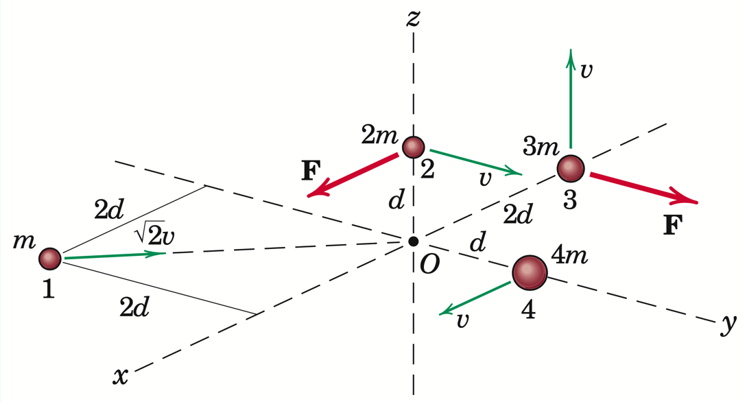
The system of four particles has the indicated masses, positions, velocities, and external forces as shown in the figure above. For now, you can ignore the forces; we will revisit this in the next week’s activities.

Your task is to compute the angular momentum of this system of particles about two points:

1. the point O.

2. the system’s mass centre (so you will have to compute this). You can assume this point is called G.

You may makes use of all the tools you have learned so far in SymPy to complete your work.

Solution Part 1: Angular Momentum of \(S\) about \(O\)

The theory

A system of particles \(S\) is provided. You are asked to compute the angular momentum of S about O: \({\bf H}^{S/O}\). In principle, this means computing the angular momentum of each particle and adding them up; this is also known as the composite theorem. This is given by:

\({\bf H}^{S/O} = \sum_{i=1}^4 {\bf H}^{P_i/O}\)

or

\({\bf H}^{S/O} = {\bf H}^{P_1/O} + {\bf H}^{P_2/O} + {\bf H}^{P_3/O} + {\bf H}^{P_4/O}\).

We also have the definition for angular momentum of a generic particle \(P_i\) about \(O\) given by:

\({\bf H}^{P_i/O} \triangleq {\bf r}^{OP_i} \times m_{P_i} ^N{\bf v}^{P_i}\)

, where:

\({\bf r}^{OP_i}\) is the position vector from a point \(O\) to \(P_i\);

\(m_{P_i}\) is the mass of \(P_i\); and

\(^N{\bf v}^{P_i}\) is the velocity of \(P_i\) with respect to a reference frame \(N\).

So, now, we can turn to the features of sympy to compute each of these angular momenta symbolically (as this problem does not assign numerical values to the mass, velocity, or position vectors). Then, we can use the composite theorem to compute the angular momentum of \(S\).

Computing the solution

from sympy import symbols, sin, cos
from sympy.physics.mechanics import ReferenceFrame, Point, dynamicsymbols
m, d, v = symbols('m d v')
N = ReferenceFrame('N')

Computing \({\bf H}^{P_1/O}\)

P1 = Point('P1')
m_P1 = m # mass of P
r_OP1 = 2*d*(N.x - N.y)
P1.set_vel(N, v*(-N.x + N.y))
N_v_P1 = P1.vel(N)
linear_momentum_of_P1 = m_P1*N_v_P1
angular_momentum_of_P1_about_O = r_OP1.cross(linear_momentum_of_P1)

Computing \({\bf H}^{P_2/O}\)

P2 = Point('P2')
m_P2 = 2*m # mass of P
r_OP2 = d*N.z
P2.set_vel(N, v*N.y)
N_v_P2 = P2.vel(N)
linear_momentum_of_P2 = m_P2*N_v_P2
angular_momentum_of_P2_about_O = r_OP2.cross(linear_momentum_of_P2)

Computing \({\bf H}^{P_3/O}\)

P3 = Point('P3')
m_P3 = 3*m # mass of P
r_OP3 = -2*d*N.x
P3.set_vel(N, v*N.z)
N_v_P3 = P3.vel(N)
linear_momentum_of_P3 = m_P3*N_v_P3
angular_momentum_of_P3_about_O = r_OP3.cross(linear_momentum_of_P3)

Computing \({\bf H}^{P_4/O}\)

P4 = Point('P4')
m_P4 = 4*m # mass of P
r_OP4 = +d*N.y
P4.set_vel(N, v*N.x)
N_v_P4 = P4.vel(N)
linear_momentum_of_P4 = m_P4 * N_v_P4
angular_momentum_of_P4_about_O = r_OP4.cross(linear_momentum_of_P4)

Computing \({\bf H}^{S/O}\)

H_of_S_about_O = angular_momentum_of_P1_about_O + angular_momentum_of_P2_about_O + angular_momentum_of_P3_about_O + angular_momentum_of_P4_about_O
H_of_S_about_O

\[\displaystyle - 2 d m v\mathbf{\hat{n}_x} + 6 d m v\mathbf{\hat{n}_y} - 4 d m v\mathbf{\hat{n}_z}\]

Solution Part 2: Angular Momentum of \(S\) about \(S^*\)

The theory

Here you are asked to compute the angular momentum of S about the system’s mass centre (let’s call it \(S^*\)): \({\bf H}^{S/S^*}\). Once again, this can be done using the composite theorem:

\({\bf H}^{S/S^*} = \sum_{i=1}^4 {\bf H}^{P_i/S^*}\),

where,

\({\bf H}^{P_i/S^*} \triangleq {\bf r}^{S{^*}P_i} \times m_{P_i} ^N{\bf v}^{P_i}\)

But, we haven’t computed \({\bf r}^{S{^*}P_i}\). This requires that we first know the location of the \(S^*\) from \(O\) using the definition of mass centres:

\({\bf r}^{OS^*}= \frac{m_{P_1}{\bf r}^{OP_1} + m_{P_2}{\bf r}^{OP_2} + m_{P_3}{\bf r}^{OP_3} + m_{P_4}{\bf r}^{OP_4}}{m_{P_1} + m_{P_2} + m_{P_3} + m_{P_4}}\).

Then, we can compute \({\bf r}^{S{^*}P_i}\) (which is needed in the computation of each particle’s angular momentum for this section) as:

\({\bf r}^{S{^*}P_i} = {\bf r}^{OP_i}- {\bf r}^{OS^*}\).

Based on this theory, we now complete the computing task as shown below:.

Computing the solution

r_OSstar = (m_P1*r_OP1 + m_P2*r_OP2 + m_P3*r_OP3 + m_P4*r_OP4)/(m_P1 + m_P2 + m_P3 + m_P4)
r_OSstar

\[\displaystyle - \frac{2 d}{5}\mathbf{\hat{n}_x} + \frac{d}{5}\mathbf{\hat{n}_y} + \frac{d}{5}\mathbf{\hat{n}_z}\]

Computing \({\bf H}^{P_1/S^*}\)

r_SstarP1 = r_OP1 - r_OSstar
angular_momentum_of_P1_about_Sstar = r_SstarP1.cross(linear_momentum_of_P1)

Computing \({\bf H}^{P_2/S^*}\)

r_SstarP2 = r_OP2 - r_OSstar
angular_momentum_of_P2_about_Sstar = r_SstarP2.cross(linear_momentum_of_P2)

Computing \({\bf H}^{P_3/S^*}\)

r_SstarP3 = r_OP3 - r_OSstar
angular_momentum_of_P3_about_Sstar = r_SstarP3.cross(linear_momentum_of_P3)

Computing \({\bf H}^{P_4/S^*}\)

r_SstarP4 = r_OP4 - r_OSstar
angular_momentum_of_P4_about_Sstar = r_SstarP4.cross(linear_momentum_of_P4)

Computing \({\bf H}^{S/S^*}\)

H_of_S_about_Sstar = angular_momentum_of_P1_about_Sstar + angular_momentum_of_P2_about_Sstar + angular_momentum_of_P3_about_Sstar + angular_momentum_of_P4_about_Sstar
H_of_S_about_Sstar

\[\displaystyle - 2 d m v\mathbf{\hat{n}_x} + \frac{21 d m v}{5}\mathbf{\hat{n}_y} - \frac{11 d m v}{5}\mathbf{\hat{n}_z}\]