Direction Cosine Matrix (DCM)

(14)\[\begin{split}\begin{bmatrix} \hat{\bf b}_x\\ \hat{\bf b}_y\\ \hat{\bf b}_z\\ \end{bmatrix} = \begin{bmatrix} \cos{\theta} & 0 & \sin\theta \\ 0 & 1 & 0 \\ -\sin\theta & 0 & \cos\theta \\ \end{bmatrix} \begin{bmatrix} \hat{\bf a}_x\\ \hat{\bf a}_y\\ \hat{\bf a}_z\\ \end{bmatrix}\end{split}\]

which can be written in short-hand as:

(15)\[\begin{split}\begin{bmatrix} \hat{\bf b}_x\\ \hat{\bf b}_y\\ \hat{\bf b}_z\\ \end{bmatrix} = {}^B\begin{bmatrix} C \end{bmatrix}^A \begin{bmatrix} \hat{\bf a}_x\\ \hat{\bf a}_y\\ \hat{\bf a}_z\\ \end{bmatrix}\end{split}\]

Continuing with the matrix representation of the door-wall example, the \(3\times3\) matrix relates the \(B\)-frame’s unit vectors to the \(A\)-frame’s unit vectors. It is called the direction cosine matrix of \(A\) in \(B\). The symbolic notation of it is\({}^B\begin{bmatrix}C\end{bmatrix}^A\). This is for a rotation about \(y\)-axis, as mentioned on the previous page.

Simple rotation about \(x\)-axis would result in the following DCM.

(16)\[\begin{split}{}^B\begin{bmatrix} C \end{bmatrix}^A = \begin{bmatrix} 1 & 0 & 0 \\ 0 & \cos{\theta} & \sin\theta \\ 0 & -\sin\theta & \cos\theta \\ \end{bmatrix}\end{split}\]

And, similarly, simple rotation about \(z\)-axis would result in the following DCM:

(17)\[\begin{split}{}^B\begin{bmatrix} C \end{bmatrix}^A = \begin{bmatrix} \cos{\theta} & \sin\theta & 0\\ -\sin\theta & \cos\theta & 0\\ 0 & 0 & 1\\ \end{bmatrix}\end{split}\]

Terminology

Why does the term Direction Cosine Matrix have the term \(\text{cosine}\) in its name?

Recall that Equation set (10) was derived purely using the \(\text{cosine}\) of angles between pairs of unit vectors. For example, consider the \(x\)-unit vector of the \(B\)-frame as represented in the \(A\)-frame:

\[ \hat{\bf b}_x = \cos{\theta}\hat{\bf a}_x + \cos{(90-0)}\hat{\bf a}_z \]

which then becomes

\[ \hat{\bf b}_x = \cos{\theta}\hat{\bf a}_x + \sin{\theta}\hat{\bf a}_z \]

This can be written in a more generic form using only dot products (as this product is defined using \(\text{cosine}\) terms), as shown below:

\[ \hat{\bf b}_x = (\hat{\bf b}_x\cdot{}\hat{\bf a}_x)\hat{\bf a}_x + (\hat{\bf b}_x\cdot{}\hat{\bf a}_y)\hat{\bf a}_y + (\hat{\bf b}_x\cdot{}\hat{\bf a}_z)\hat{\bf a}_z \]

where,

\[ \hat{\bf b}_x\cdot{}\hat{\bf a}_y = \cos{90^{\circ}} = 0 \]

This serves as the foundation for a more general description of orientations for General \(3D\) Rotation.

General \(3D\) Rotation and DCM

Below, body \(B\) is moving freely relative to frame \(A\):

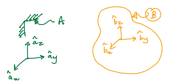
From the preceding discussion on dot products and DCM, we can write the following relationships between two reference frame \(A\) and \(B\).

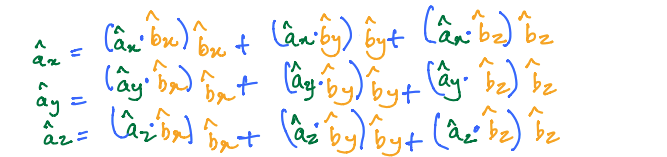
The above equation can also be written in its matrix form as:

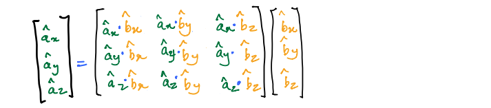
which can also be written more succinctly (and, this time, in typeface) as:

(18)\[\begin{split}\begin{bmatrix} \hat{\bf a}_x\\ \hat{\bf a}_y\\ \hat{\bf a}_z\\ \end{bmatrix} = {}^A\begin{bmatrix} C \end{bmatrix}^B \begin{bmatrix} \hat{\bf b}_x\\ \hat{\bf b}_y\\ \hat{\bf b}_z\\ \end{bmatrix}\end{split}\]

\({}^A\begin{bmatrix}C\end{bmatrix}^B\) is the direction \(\text{cosine}\) matrix of \(B\) in \(A\).

Note

\({}^{A}\begin{bmatrix}C\end{bmatrix}^{B} \neq {}^{B}\begin{bmatrix}C\end{bmatrix}^{A}\)

A key property of DCM

A very important property of DCM is that it is an orthogonal matrix. Mathematically, this means that the inverse of the DCM is the same as the transpose of the matrix. In other words, if the DCM is given by a matrix \(\begin{bmatrix}M\end{bmatrix}^{B}\), then:

(20)\[\begin{bmatrix}M\end{bmatrix}^{-1} = \begin{bmatrix}M\end{bmatrix}^{T}\]

This is a very useful result because it is considerably easier to compute the transpose of a matrix than it is to compute its inverse.

How is this property useful?:

At this point, we know that we can express the same vector in different reference frames. This property allows us to do so in a very easy manner. Below we show how you can easily convert (or express) a vector given in the \(B\)-frame to its equivalent in the \(A\)-frame.

(20)\[\begin{split}\begin{bmatrix} \hat{\bf a}_x\\ \hat{\bf a}_y\\ \hat{\bf a}_z\\ \end{bmatrix} = {}^A\begin{bmatrix} C \end{bmatrix}^B \begin{bmatrix} \hat{\bf b}_x\\ \hat{\bf b}_y\\ \hat{\bf b}_z\\ \end{bmatrix} \longrightarrow \begin{bmatrix} \hat{\bf b}_x\\ \hat{\bf b}_y\\ \hat{\bf b}_z\\ \end{bmatrix} = ({}^A\begin{bmatrix} C \end{bmatrix}^B)^{-1} \begin{bmatrix} \hat{\bf a}_x\\ \hat{\bf a}_y\\ \hat{\bf a}_z\\ \end{bmatrix} \longrightarrow \begin{bmatrix} \hat{\bf b}_x\\ \hat{\bf b}_y\\ \hat{\bf b}_z\\ \end{bmatrix} = ({}^A\begin{bmatrix} C \end{bmatrix}^B)^{T} \begin{bmatrix} \hat{\bf a}_x\\ \hat{\bf a}_y\\ \hat{\bf a}_z\\ \end{bmatrix}\end{split}\]

In fact, when one compares Equaitons (20) and (15) one sees that:

(21)\[{}^B\begin{bmatrix} C \end{bmatrix}^A = ({}^A\begin{bmatrix} C \end{bmatrix}^B)^{T}\]