Kinetics

You may recall that dynamics was principally divided into two key parts: kinematics and kinetics. If you’ve followed along this far, here’s a recap of our journey:

1. We have already examined kinematics in some detail. One must pause to take note here that, in this case, motion was investigated without considering the forces causing it.

2. Then, we introduced concepts such as mass/inertia scalars.

3. Next we focused on forces; moments; and the various types of momenta.

This leads up to the final act: kinetics, which is the piece of the puzzle that relates the causes of motion (forces and moments) to the bodies. The law that connects them is one that you are likely already familiar with - Newton’s Second Law. Quite simply put, this law states that the acceleration of a particle \(P\) (for now, denoted as \(\mathbf{a}\)) is directly proportional to the force \(\mathbf{F}\) acting on it. One may have also seen this law written as the following equation:

(40)\[{\mathbf F} = m{\mathbf a}\]

In the following discussion, we dive deeper into this equation. A keen reader of this text may have already taken note that the vectors written here are incomplete when compared to our approach so far, i.e., our typical vector notations make use of super-scripts (and subscripts, in some cases) to specify reference frames, particles, bodies, etc.

Key Concept: Inertial Frame

In our discussions within kinematics, we have described positions in space of objects (i.e., points and reference frames) relative to some other reference frame by means of linear and angular measurements. In many cases, we made use of reference frames that were fixed (i.e., the ground).

Newton’s laws of mechanics are valid in a frame known as an inertial reference frame (or inertial frame or Newtonian frame).

• Definition 1: Textbooks often define something known as a primary inertial system, which is a reference frame that is neither translating nor rotating in space. The laws of Newton are said to hold in this frame; experiments show that the laws are valid in such a frame as long as the velocities involved are negligible compared with the speed of light, which is 300,000 km/s. Consequently, for several engineering problems, the Earth can be approximated to an inertial frame in studying the motion of objects moving on it (like cars) and close to it (spacecraft in Low Earth Orbit).

• Definition 2: It is also seen that Newton’s laws hold in any non-rotating reference frame that moves with a constant velocity; the time derivative of a constant velocity leads to zero acceleration. Thus, another definition emerges for an inertial frame as a frame which has zero acceleration (or is a non-accelerating reference frame).

As a result of the two definitions above, you will also commonly see books define an inertial frame in a rather circuitous manner as a frame in which Newton’s second law is valid. Now you know why.

Equations of motion

Newton’s second law (as stated above) is a vector equation; indeed, they can be written as 3 scalar equations called Equations of Motion.

\[\begin{split} \mathbf{{F}} = m\mathbf {{a}} \Longrightarrow \begin{cases} \mathbf{F_x} = m\mathbf{a_x} \\ \mathbf{F_y} = m\mathbf{a_y} \\ \mathbf{F_z} = m\mathbf{a_z} \\ \end{cases} \end{split}\]

The above equations can be used to solve two types of problems:

• Acceleration is known and we have to calculate the forces: Acceleration is either specified or can be determined directly from known kinematic conditions. The corresponding forces on the particle can then be directly determined from Newton’s Second Law.

• Forces are known and motion needs to be determined:

  • Case 1: If the forces are constant, the acceleration is also constant and is easily found using the equations of motion.

  • Case 2: In the most general case, forces are functions of time, position, or velocity; so the above set of equations are differential equations. These are more challenging problems. Deriving these general equations is the goal of this portion of the module.

Free body diagrams to determine forces

• Developing equations of motion requires that you account correctly for all forces acting on any object.

• The only reliable way to account for every force is to isolate the particle under consideration from all contacting and influencing bodies and replace the bodies removed by the forces they exert on the particle isolated.

Attention

Note that not all the forces are known in terms of their magnitude e.g., reaction forces (this will become clearer later); but we need to account for all forces at a qualitative level in our free-body diagram.

The types of forces to account for are:

Gravitational Forces:

The gravitational force between two masses is given by:

\[ F = \frac{Gm_1m_2}{r^2} \]

where \(G\) is the gravitational constant, \(m_1\) and \(m_2\) are the masses of the objects, and \(r\) is the distance between their centers.

Friction Forces:

• Dynamic friction forces are those that oppose the movement of an object already in motion. They are generally less than static friction forces and are described by:

  \[ F_{\text{dynamic}} = \mu_d N \]

  where \(\mu_d\) is the coefficient of dynamic friction and \(N\) is the normal force.

• Static friction forces prevent an object from moving while it is at rest. The maximum static friction force is given by:

  \[ F_{\text{static}} \leq \mu_s N \]

  where \(\mu_s\) is the coefficient of static friction.

Spring Forces:

The force exerted by a linear spring is described by Hooke’s Law:

\[ F = -k x \]

where \(k\) is the spring constant and \(x\) is the displacement from the equilibrium position.

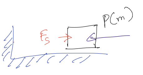
Fig. 16 Spring forces

Types of motion

There are two physically distinct types of motion:

• Unconstrained motion: where the moving object is free of mechanical guides and follows a path determined by its initial motion and by the forces which are applied to it from external sources. An example here is the motion of a satellite or a rocket in flight.

• Constrained motion: where the moving object is partially or totally restrained by guides. Thus, in addition to external forces, there are also reaction forces that emerge. An example of fully constrained motion is of a train moving along a track. The motion of a car is another example as it is constrained to move on the horizontal plane.

Kinetics of a Single Particle: Unconstrained Motion

For a particle \(P\), moving relative to a frame \(N\) under the influence of an external force \(F\), we have Newton’s second law:

\[\mathbf{{F}} = m^{N}\mathbf{{a}}^P\]

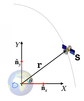
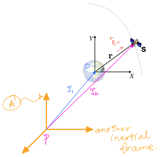
Practical example: The case of motion of a \(S\), a spacecraft, about the Earth:

Attention

GOAL: To find the equations of motion of \(S\).

Prior to any equations, each term required must be defined.

\(m_1\) = Mass of the Earth

\(m_2\) = Mass of the Spacecraft

\(\mathbf{{r}}\) = Position vector from \(O\) to \(S\)

\(\theta\) = Inclination of position vector

\(N\) = Earth’s inertial reference frame

Free Body Diagram

Using Cartesian coordinates the position and velocity vectors can be defined.

\[\mathbf{{r}} = x\hat{\mathbf n_x}+y\hat{\mathbf n_y}\]

\[{}^{N}{\mathbf{{v}}}^{S} = \frac{{}^N d} {\mathrm{d}t} \mathbf{{r}} = \dot{x}\hat{\mathbf n_x}+\dot{y}\hat{\mathbf n_y}\]

The acceleration vector can then be defined as:

\[{}^{N}{\mathbf{{a}}}^{S} = \frac{{}^N d} {\mathrm{d}t}{}^{N}{\mathbf{{v}}}^{S} = \frac{{}^N d} {\mathrm{d}t}(\dot{x}\hat{\mathbf n_x}+\dot{y}\hat{\mathbf n_y})\]

\[{}^{N}{\mathbf{{a}}}^{S} = \ddot{x}\hat{\mathbf n_x}+\ddot{y}\hat{\mathbf n_y}\]

\[{F_g}=\frac{G{m_1}{m_2}}{|\mathbf{{r}}|^{2}}\]

\[\mathbf{{F}} = -{F_g}(cos\theta\hat{\mathbf n_x}+sin\theta\hat{\mathbf n_y})\]

From this it can be seen that \(\mathbf{{F}} = m\mathbf{{a}}\) gives two scalar equations - displayed below.

x Direction:

\[-{F_g}cos\theta = \ddot{x}{m_2}\]

y Direction:

\[-{F_g}sin\theta = \ddot{y}{m_2}\]

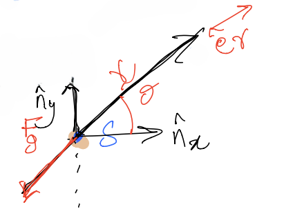
Now, making use of Polar Coordinates…

\[\mathbf{{r}}=r{\hat{\mathbf e_r}}\]

\[{}^{N}\mathbf{{v}}^{S} \triangleq \frac{{}^N d} {\mathrm{d}t}{}^{N}\mathbf{{r}}^{S} = \frac{{}^N d} {\mathrm{d}t}r{\hat{\mathbf e_r}}\]

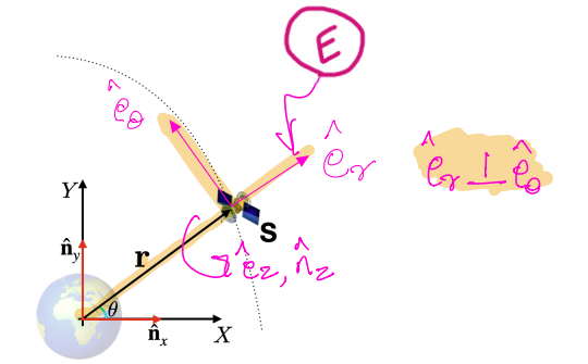
The velocity vector,\({}^{N}\mathbf{{v}}^{S}\) , can be determined as:

\[{}^{N}\mathbf{{v}}^{S} \triangleq \frac{{}^N d} {\mathrm{d}t}{}^{N}\mathbf{{r}}^{S} = {}^{N}{\frac d {\mathrm{d}t}}r{\hat{\mathbf e_r}}\]

\[= \frac{{}^E d} {\mathrm{d}t}(r{\hat{\mathbf e_r}})+{}^{N}\boldsymbol{{\omega}}^{E} \times r{\hat{\mathbf e_r}}\]

\[= \dot{r}{\hat{\mathbf e_r}}+\dot{\theta}{\hat{\mathbf e_z}} \times {r}{\hat{\mathbf e_r}}\]

\[= \dot{r}{\hat{\mathbf e_r}}+r\dot{\theta}{\hat{\mathbf e_\theta}}\]

The acceleration vector,\({}^{N}\mathbf{{a}}^{S}\), can be determined as:

\[{}^{N}\mathbf{{a}}^{S} = \frac{{}^N d} {\mathrm{d}t}\mathbf{{v}}^{S} = \frac{{}^E d} {\mathrm{d}t}{}^{N}\mathbf{{v}}^{S} + {}^{N}\boldsymbol{{\omega}}^{E} \times {}^{N}\mathbf{{v}}^{S}\]

\[= \frac{{}^E d} {\mathrm{d}t}(\dot{r}{\hat{\mathbf e_r}} + {r}\dot{\theta}{\hat{\mathbf e_\theta}}) + \dot{\theta}{\hat{\mathbf e_z}} \times (\dot{r}{\hat{\mathbf e_r}} + {r}\dot{\theta}{\hat{\mathbf e_\theta}})\]

\[{}^{N}\mathbf{{a}}^{S} = (\ddot{r}-r{\dot{\theta}^2}){\hat{\mathbf e_r}} + (2\dot{r}\dot{\theta}+r\ddot{\theta})\hat{\mathbf e_\theta}\]

Next, since \(\mathbf{{F}} = {m_2} {}^{N}\mathbf{{a}}^{S}\) for this satellite…

\[-F_g = {m_2}(\ddot{r}-\dot{r}\theta^2) \rightarrow \hat{\mathbf e_r} \text{ direction}\]

\[0 = {m_2}(2{\dot{r}\dot{\theta}}-{r}\ddot{\theta}) \rightarrow \hat{\mathbf e_\theta} \text{ direction}\]

The force equations for the Earth and satellite can be given as follows:

For the Earth:

\[\mathbf{{F}_{Earth}} = {m_1} \frac{{}^A d^2} {\mathrm{d}t^2}\mathbf{{r}_{1}} = m_1\ddot{\mathbf{{r}}}_{1} + {F_g}{\hat{\mathbf e_r}} = m_1\ddot{\mathbf{{r}}}_{1}\]

For the Spacecraft:

\[\mathbf{{F}_{Spacecraft}} = {m_2} \frac{{}^A d^2} {\mathrm{d}t^2}\mathbf{{r}_{2}} = m_2\ddot{\mathbf{{r}}}_{2} - {F_g}{\hat{\mathbf e_r}} = m_2\ddot{\mathbf{{r}}}_{2}\]

Now you can add both equations. This gives a combined force equation equal to zero:

\[{F_g}{\hat{\mathbf e_r}} - {F_g}{\hat{\mathbf e_r}} = m_1\ddot{\mathbf{{r}}}_{1} + m_2\ddot{\mathbf{{r}}}_{2}\]

\[ 0 = m_1\ddot{\mathbf{{r}}}_{1} + m_2\ddot{\mathbf{{r}}}_{2}\]

Hint

Recall that, systems of particles have a fictitious point called the mass centre; let’s call it \(G\) in this case (see figure). In this scenario, we have the definition of the mass centre as:

\[{m_1} {\mathbf{{r}}}_{1} + {m_2} {\mathbf{{r}}}_{2} = \left(\sum_{i=1}^2 m_i\right) {\mathbf{{r}}}_{G}\]

Consequently, we can get:

\[{m_1} \frac{{}^A d} {\mathrm{d}t} \mathbf{{r}} {\mathbf{{r}}}_{1} + {m_2} \frac{{}^A d} {\mathrm{d}t} {\mathbf{{r}}}_{2} = \left(\sum_{i=1}^2 m_i\right) \frac{{}^A d} {\mathrm{d}t} {\mathbf{{r}}}_{G}\]

And:

\[{m_1} \frac{{}^A d} {\mathrm{d}t} {\mathbf{{r}}}_{1} + {m_2} \frac{{}^A d} {\mathrm{d}t} {\mathbf{{r}}}_{2} = \left(\sum_{i=1}^2 m_i\right) \frac{{}^A d} {\mathrm{d}t} {\mathbf{{r}}}_{G}\]

\[{m_1} \frac{{}^A d^2} {\mathrm{d}t} {\mathbf{{r}}}_{1} + {m_2} \frac{{}^A d^2} {\mathrm{d}t} {\mathbf{{r}}}_{2} = \left(\sum_{i=1}^2 m_i\right) \frac{{}^A d^2} {\mathrm{d}t} {\mathbf{{r}}}_{G} \tag{11.2}\]

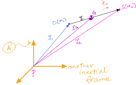
Equation \(11.2\) can be rewritten using \(11.1\) as:

\[\left(\sum_{i=1}^2 m_i\right) {}^{A}{\mathbf{{a}}}_{G}\]

or:

\[{}^{A}{\mathbf{{a}}}_{G} = 0\]

Which also implies:

\[{}^{A}{\mathbf{{v}}}_{G} = \text{constant}\]

In this second discussion, we have considered the motion of a system containing two particles: one being the spacecraft and the other being the Earth. First, we studied the motion of each particle from an inertial frame. Subsequently, we combined this information to study the motion of the two-particle system from its combined mass centre, denoted as \(G\).

It turns out that this development of Newton’s second law for two-particles actually generalizes to a system comprising \(n\) particles and also to a rigid body. We examine this further in teh following section.

Generalized Newton’s Second Law

Consider a system of \(n\) particles and an inertial frame \(N\). Each particle experiences an external resultant force and a set of internal forces. The internal forces are reaction forces applied by each particle on all other particles within the boundary.

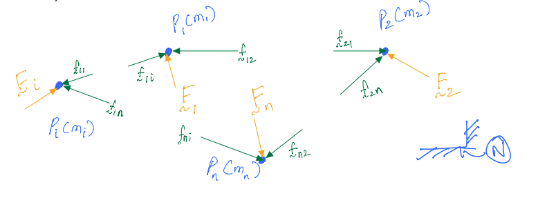
We can now write the equations of motion for each of the particles:

For \(\mathbf{P_1}\)

\[{\mathbf{{F}}_1} + {\mathbf{{f}}_12} + {\mathbf{{F}}_1n} + {\mathbf{{F}}_1i} = {m_1}{}^{N}{\mathbf{a}}^{p_1}\]

\[{\mathbf{{F}}_1} + \sum_{k=1}^n {\mathbf{{f}}_{1k}} = {m_1}{{}^{N}{\mathbf{{a}}}^{p_1}} \tag{11.3}\]

For \(\mathbf{P_2}\)

\[{\mathbf{{F}}_2} + \sum_{k=1}^n {\mathbf{{f}}_{2k}} = {m_2}{{}^{N}{\mathbf{{a}}}^{p_2}} \tag{11.4}\]

For \(\mathbf{P_i}\)

\[{\mathbf{{F}}_i} + \sum_{k=1}^n {\mathbf{{f}}_{ik}} = {m_i}{{}^{N}{\mathbf{{a}}}^{p_i}} \tag{11.5}\]

For \(\mathbf{P_n}\)

\[{\mathbf{{F}}_n} + \sum_{k=1}^n {\mathbf{{f}}_{nk}} = {m_n}{{}^{N}{\mathbf{{a}}}^{p_n}}\tag{11.6}\]

We can now add up all the equations form \(11.3\) to \(11.6\) to get…

\[\sum_{k=1}^n {\mathbf{{f}}_{k}} + \sum_{j=1}^n {\mathbf{{f}}} \sum_{k=1}^n {\mathbf{{f}}_{jk}} = \sum_{k=1}^n ({m_k}{{}^{N}{\mathbf{{a}}}^{p_k}}) \tag{11.6}\]

Where:

• \(\sum_{k=1}^n {\mathbf{{f}}_{k}}\) is the resultant external force on the system.

• \(\sum_{j=1}^n {\mathbf{{f}}} \sum_{k=1}^n {\mathbf{{f}}_{jk}}\) is the sum of all internal forces.

If the sum of all internal forces is deemed to be zero..

\[\sum_{k=1}^n {\mathbf{{f}}_{k}} + \cancel{\sum_{j=1}^n {\mathbf{{f}}} \sum_{k=1}^n {\mathbf{{f}}_{jk}}} = \sum_{k=1}^n ({m_k}{{}^{N}{\mathbf{{a}}}^{p_k}})\]

So,

\[\sum_{k=1}^n {\mathbf{{f}}_{k}} = \sum_{k=1}^n ({m_k}{{}^{N}{\mathbf{{a}}}^{p_k}})\]

Or,

\[\sum_{k=1}^n {\mathbf{{f}}_{k}} = \left(\sum_{k=1}^n {m_k}\right) {{}^{N}{\mathbf{{a}}}^{S^*}}\]

\[{\mathbf{{f}}} = {m} {{}^{N}{\mathbf{{a}}}^{S^*}}\]

Where \(S^*\) is the mass centre of the system of particles.

So far, everything we have studied addresses the kinetics of a point mass; the point mass was either a particle (e.g., a satellite) or a mass centre of a system of particles. This only describes the translational motion or the translational dynamics, which is based on Newton’s second law (the time derivative of linear momentum is equal to forces acting on a system). So what about the rotational dynamics?