JN4: Practice Activity 3#
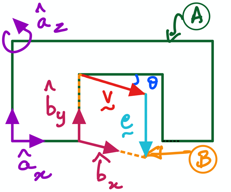
Fig. 7 Motion of a door \(B\) relative to wall \(A\).#
This activity returns to the door-wall example (see figure above); it also utilises code first written in PA1 to teach you how to use direction cosine matrices to support your work as a dynamics engineer.
This notebook has three objectives:
creating a Direction Cosine Matrix (DCM) and using it to configure the orientation between two reference frames \(A\) and \(B\) using
sympy; andobtaining angular velocity and angular accelerations using
sympy; anda method of expressing any vector in different frames with
sympywhich works once the DCM is known.
The code in Section 2 is to express vectors \(\bf v\) and \(\bf e\) in the \(B\)-frame; in other words, it is a repeat of PA1 . Sections 3, 4, and 5 address the 3 objectives above.
Pre-work from JN1#
Create scalars using symbols and dynamicsymbols#
from sympy import symbols
from sympy.physics.mechanics import dynamicsymbols, ReferenceFrame
v, e = symbols('v e')
theta = dynamicsymbols('theta')
---------------------------------------------------------------------------
ModuleNotFoundError                       Traceback (most recent call last)
Cell In[1], line 1
----> 1 from sympy import symbols
      2 from sympy.physics.mechanics import dynamicsymbols, ReferenceFrame
      3 v, e = symbols('v e')

ModuleNotFoundError: No module named 'sympy'
Creating Reference Frames#
A and B are reference frames. Let’s create them using SymPy!
A = ReferenceFrame('A')
B = ReferenceFrame('B')
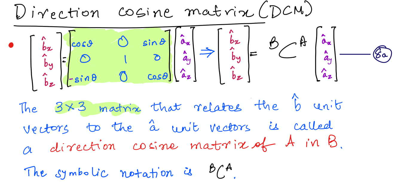
Direction Cosine Matrices for Orienting Reference Frames#
We now have created the vectors \(\bf v\) and \(\bf e\) in component form in the \(B\)-system; they are stored in variables named v_vec and e_vec. Recall from PA2 that we had used variables named v_vec_B and e_vec_B for this purpose. Then, we introduced variable names v_vec_A and e_vec_A when \(\bf v\) and \(\bf e\) were expressed in the \(A\) frame. This was done for good bookkeeping. However, we know that v_vec_A and v_vec_b are the same vector \(\bf v\)! (All of this is also true for \(\bf e\) and its variables e_vec_A and e_vec_B.)
Question: How did we convert vectors \(\bf v\) and \(\bf e\) given in B-frame unit vectors to to A-frame unit vectors?
Answer: Using Direction Cosine Matrices, \(^B\mathbf{C}^A\), to rotate \(B\) relative to \(A\) (see below: Equation 8a from file ‘ 4 rigid body kinematics: orientations.pdf’).
Now, we must ask ourselves (or might already have questioned):
How can we exploit
sympyto convert the vectors while minimizing hand computation?Answer: We can do this in two steps:
Step 1: create a \(^B\mathbf{C}^A\) using the
Matrixfeature ofsympy; andStep 2: use the DCM created in Step 1 in the
orientmethod to correctly perform the rotation ofBrelative toA.
The implementation of this is explained below.
Step 1: Creating \(^A\mathbf{C}^B\) withsympy#
To create any matrix using, we must first import the Matrix feature from sympy as below (we import sin and cos as well because we know the Matrix requires it):
from sympy import Matrix, sin, cos
We will use the variable name B_dcm_A to store the direction cosine matrix \(^B\mathbf{C}^A\).
B_dcm_A = Matrix([
    [cos(theta), 0, sin(theta)],
    [0, 1, 0],
    [-sin(theta), 0, cos(theta)]
])
We can examine the contents of the B_dcm_A:
B_dcm_A
Use B_dcm_A and orient method of frame A to rotate B#
We can now orient A and B using the orient method with the DCM with the following line of code:
A.orient(B, 'DCM', B_dcm_A)
In this case, the orient method takes the following sequence of information in the parantheses:
Frame of rotation, in this case,
Bthe type of rotation, in this case it is the
DCM(later in PA5, we will useAxisas another way of defining rotations); and
the specific matrix that we are using as the DCM. In this case, it is
B_dcm_A.
__ You will get an error (or incorrect result) if you do not provide the information in the order listed above or give it incorrect information__.
It is easy to determine the expressions for \(^A\omega^B\) and \(^A\alpha^B\) by examining the figure and writing it out by hand. This can also serve as the sanity check for the results produced by sympy for these vectors by examining the angular velocity and angular acceleration of B in A, with the following two lines of code:
B.ang_vel_in(A)
B.ang_acc_in(A)
How can we express vectors in different frames with sympy and B_dcm_A that we created above?#
Create the vectors in B-frame (slightly modified from PA1)#
In this section, we use the variable names v_vec and e_vec for \(\bf v\) and \(\bf e\); we write the vectors in the B reference frame.
v_vec = v*B.x
e_vec = -e*B.y
We append the .express method to a variable representing a Vector to automatically convert it into a new frame:
v_vec.express(A)
Exercsie: Can you write the same for the vector \(\bf e\)?#
Can you define the vector \(\bf e\) expressed in the unit vectors attached to the frame A? You should use a variable name e_vec_A to do so in the cell below: