Table of Contents
Problem 3: Angular Momentum of Rigid Body#
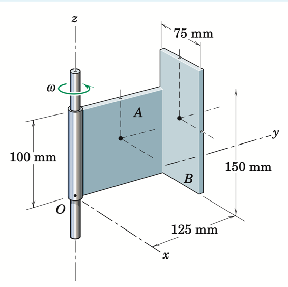
Fig. 15 Door wall#
The bent plate has a mass of 70 kg per square meter of surface area and re-volves about the z-axis at the rate 30 rad/s. Determine the angular momentum of the plate about point O.
Solution#
The theory#
The figure above shows a bent plate comprising two rigid bodies, \(A\) and \(B\). Since \(A\) and \(B\) are rigidly attached to each other, you can even say that the plate is one body which we refer to as S from hereon.
You are asked to compute the angular momentum of this bent plate, S, about O: \({\bf H}^{S/O}\). Note that \(O\) is a point fixed both in \(S\) and \(N\).
So, we can compute \({\bf H}^{S/O}\) from equation 10.5 in the file titled “10 momentum: linear and angular”, which gives the angular momentum of an arbitrary body \(B\) about a point \(Q\) fixed in \(B\). We repeat this equation below:
\( {\bf H}^{B/Q} = {\bf r}^* \times m ^N{\bf v}^Q + [{\bf I}]^{B/Q} {^N}\omega^B\)
, where
\([{\bf I}]^{B/Q}\) is the inertia matrix of \(B\) about \(Q\). In the assigned problem, the point \(O\) is analogous to \(Q\) and \(S\) is analogous to \(B\).
So for this particular problem, we can recast the above equation as: \( {\bf H}^{S/O} = {\bf r}^* \times m ^N{\bf v}^O + [{\bf I}]^{S/O} {^N}\omega^S\)
Notice from the figure that \(O\) is also fixed in \(N\). So, we get \(^N{\bf v}^O = 0\) in the preceding equation which then reduces to:
\( {\bf H}^{B/Q} = [{\bf I}]^{S/O} {^N}\omega^S\).
This is a manageable problem. So, now, we have to do two things:
Compute \([{\bf I}]^{S/O}\): This can be done by first using composite theorem as \(S\) is made of two rectangular plates \(A\) and \(B\). Then, we use parallel axis theorem on each plate.
Evaluate \( {^N}\omega^S\): This is trivial as we are already told that the bent plate is rotating at \(30\) \(rad/s\). The direction of rotation is also indicated in the figure from which we deduce:
\({^N}\omega^S = 30 \hat{{\bf n}_z}\).
So, now, we can turn to the features of sympy to compute \({\bf H}^{S/O}\) as shown below.
Computational Solution#
from sympy import symbols, sin, cos, Matrix
from sympy.physics.mechanics import ReferenceFrame, Point, dynamicsymbols
---------------------------------------------------------------------------
ModuleNotFoundError                       Traceback (most recent call last)
Cell In[1], line 1
----> 1 from sympy import symbols, sin, cos, Matrix
      2 from sympy.physics.mechanics import ReferenceFrame, Point, dynamicsymbols

ModuleNotFoundError: No module named 'sympy'
Initial setup#
As the density of the plate is given and area of the sections A and B are given, we can easily compute the masses of A and B, respectively. The masses are stored in variables named m_A and m_b.
m_A = 70*(.125)*(.1) # in kg
m_B = 70*(.075)*(.15) # in kg
The figures tells us the dimensions of the plates \(A\) and \(B\) in \(mm\). However, we must use SI units in all our calculations so I convert each dimension into \(m\). I store these dimensions in the variables as described below:
l_Ais the length of plate A;b_Ais the width of plate A;l_Bis the length of plate B; andb_Bis the width of plate A.
l_A = .125 # length of plate A in m
b_A = .1 # width of A in m
l_B = 0.075 # length of B in m
b_B = .15 # width of B in m
Then, we create two reference frames \(S\) and \(N\) to store the angular velocity dedcued above. This angular velocity of S in N is stored in N_omega_S.
N = ReferenceFrame('N')
S = ReferenceFrame('S')
S.set_ang_vel(N, 30*N.z)
N_omega_S = S.ang_vel_in(N)
N_omega_S
Now, N_omega_S is a vector in its component-form but it needs to be multiplied with an inertia matrix to compute angular momentum. So we will store it as a column vector. sympy allows us to convert N_omega_S to such a form by using the .to_matrix form. This is shown below:
N_omega_S.to_matrix(N)
As you can see, we provide the frame N as to .to_matrix because N_omega_S is express in \(N\). As we need this matrix form of N_omega_S for later computations, we store it as shown below in the variable name N_omega_S_columnVector:
N_omega_S_columnVector = N_omega_S.to_matrix(N)
Evaluate inertia matrix of \(A\) about \(O\)#
O = Point('O')
#
Astar = Point('Astar')
Astar.set_pos(O, l_A/2*N.y + b_A/2*N.z)
r_OAstar = Astar.pos_from(O)
Ixx_A_about_Astar = m_A * (l_A**2 + b_A**2)/12
Iyy_A_about_Astar = m_A * (b_A**2)/12
Izz_A_about_Astar = m_A * (l_A**2)/12

I_matrix_of_A_about_A_star = Matrix([
    [Ixx_A_about_Astar, 0, 0],
    [0, Iyy_A_about_Astar, 0],
    [0, 0, Izz_A_about_Astar]
])
I_matrix_of_A_about_A_star
Ixx_Astar_about_O = m_A * (r_OAstar.cross(N.x)).dot(r_OAstar.cross(N.x))
Iyy_Astar_about_O = m_A * (r_OAstar.cross(N.y)).dot(r_OAstar.cross(N.y))
Izz_Astar_about_O = m_A * (r_OAstar.cross(N.z)).dot(r_OAstar.cross(N.z))
Ixy_Astar_about_O = m_A * (r_OAstar.cross(N.x)).dot(r_OAstar.cross(N.y))
Iyz_Astar_about_O = m_A * (r_OAstar.cross(N.y)).dot(r_OAstar.cross(N.z))
Izx_Astar_about_O = m_A * (r_OAstar.cross(N.z)).dot(r_OAstar.cross(N.x))

I_matrix_of_A_star_about_O = Matrix([
    [Ixx_Astar_about_O, Ixy_Astar_about_O, Izx_Astar_about_O],
    [Ixy_Astar_about_O, Iyy_Astar_about_O, Iyz_Astar_about_O],
    [Izx_Astar_about_O, Iyz_Astar_about_O, Izz_Astar_about_O]
])
# Parallel Axis theorem for A and B
I_matrix_of_A_about_O = I_matrix_of_A_about_A_star + I_matrix_of_A_star_about_O
I_matrix_of_A_about_O
Evaluate inertia matrix of \(B\) about \(O\)#
#
Bstar = Point('Bstar')
Bstar.set_pos(O, l_B/2*N.x + l_A*N.y + b_B/2 * N.z)
r_OBstar = Bstar.pos_from(O)

Ixx_B_about_Bstar = m_B * (b_B**2)/12
Iyy_B_about_Bstar = m_B * (l_B**2 + b_B**2)/12
Izz_B_about_Bstar = m_B * (l_B**2)/12

I_matrix_of_B_about_B_star = Matrix([
    [Ixx_B_about_Bstar, 0, 0],
    [0, Iyy_B_about_Bstar, 0],
    [0, 0, Izz_B_about_Bstar]
])
Ixx_Bstar_about_O = m_B * (r_OBstar.cross(N.x)).dot(r_OBstar.cross(N.x))
Iyy_Bstar_about_O = m_B * (r_OBstar.cross(N.y)).dot(r_OBstar.cross(N.y))
Izz_Bstar_about_O = m_B * (r_OBstar.cross(N.z)).dot(r_OBstar.cross(N.z))
Ixy_Bstar_about_O = m_B * (r_OBstar.cross(N.x)).dot(r_OBstar.cross(N.y))
Iyz_Bstar_about_O = m_B * (r_OBstar.cross(N.y)).dot(r_OBstar.cross(N.z))
Izx_Bstar_about_O = m_B * (r_OBstar.cross(N.z)).dot(r_OBstar.cross(N.x))

I_matrix_of_B_star_about_O = Matrix([
    [Ixx_Bstar_about_O, Ixy_Bstar_about_O, Izx_Bstar_about_O],
    [Ixy_Bstar_about_O, Iyy_Bstar_about_O, Iyz_Bstar_about_O],
    [Izx_Bstar_about_O, Iyz_Bstar_about_O, Izz_Bstar_about_O]
])
# Parallel Axis theorem for A and B
I_matrix_of_B_about_O = I_matrix_of_B_about_B_star + I_matrix_of_B_star_about_O
I_matrix_of_B_about_O
Composite Theorem for system’s inertia about O#
I_matrix_of_S_about_O = I_matrix_of_A_about_O + I_matrix_of_B_about_O
I_matrix_of_S_about_O
Compute \({\bf H}^{S/O}\)#
H_of_S_about_O = I_matrix_of_S_about_O*N_omega_S_columnVector
H_of_S_about_O
Key Question#
How do we know which unit vectors to use to express \({\bf H}^{S/O}\) in its component form?
Recall that:
\(^N \omega^B\) was derived in the \(N\) frame.
The inertia scalars were also computed using unit vectors attached to the \(N\) frame.
So, \({\bf H}^{S/O}\) must be expressed in the \(N\) frame.