JN7: Practice Activity 6

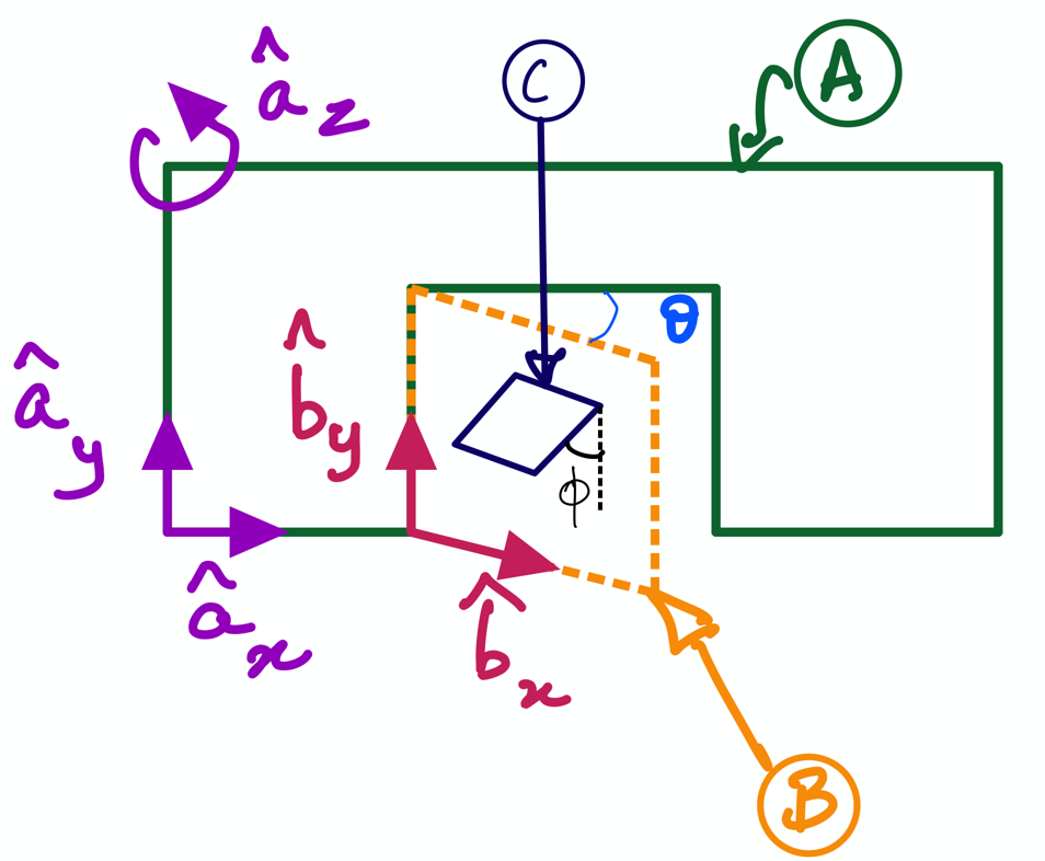
Fig. 11 Motion of catflap \(C\) relative to the door \(B\) and wall \(A\).

This notebook extends the the door-wall example (see Fig. 11) by introducing a cat flap \(C\). It is attached to the door \(B\) and makes an angle of \(\theta\) with the vertical of \(B\) (i.e. \(\hat{\bf b}_y\)). Activity L3PA4 is to find angular acceleration of the cat flap C with respect to A, i.e., \(^A\alpha^C\). Which is also shown at the very end of the file “6 Rigid body kinematics: angular velocities and angular accelerations.pdf”

Create time-varying scalars using dynamicsymbols

As was explained in L3PA1, the angle \(\theta\) between \(A\) and \(B\) changes with time. Similarly, the angle \(\phi\) between \(B\) and \(C\) also changes with time. Thus, we create both using dynamicsymbols as shown below:

from sympy.physics.mechanics import dynamicsymbols, ReferenceFrame
from sympy import sin, cos
theta, phi = dynamicsymbols('theta phi')
thetadot, phidot = dynamicsymbols('theta phi',1) # gives the first time derivative of the angles

We can examine the variables thetadot and phidot to ensure that they are time derivatives of theta and phi:

thetadot

\[\displaystyle \frac{d}{d t} \theta{\left(t \right)}\]

phidot

\[\displaystyle \frac{d}{d t} \phi{\left(t \right)}\]

Creating Reference Frames for \(A, B,\) and \(C\)

This is a trivial step at this point as we have learned how to create reference frames:

A = ReferenceFrame('A') # wall frame
B = ReferenceFrame('B') # door frame
C = ReferenceFrame('C') # cat flap frame

Computing \(^A\alpha^C\)

Approach 1: \(^A\alpha^C \triangleq \frac{^A d}{dt}\bf ^A\omega^C\)

This subsection implements the first approach of computing \(^A\alpha^C\) using \(^A\omega^C\), which must expressed in the A-frame so that the derivative can be computed.

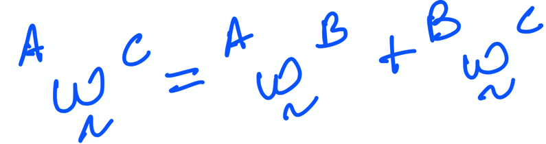
First, we must compute \(^A\omega^C\) using the chain rule:

The table below shows the mapping used between math symbols and their equivalent variable names for computing with sympy. Please note that we append _approach1 for good bookkeeping as we are going to use other approaches:

Mathematical Symbol	Equivalent Variable Name
\(^A\omega^B\)	A_omega_B_approach1
\(^B\omega^C\)	B_omega_C_approach1
\(^A\omega^C\)	A_omega_C_approach1
\(^A\omega^C\)	B_alpha_C_approach1

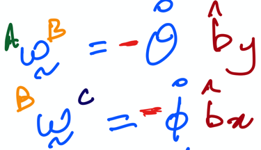
From the lecture notes, we have the following:

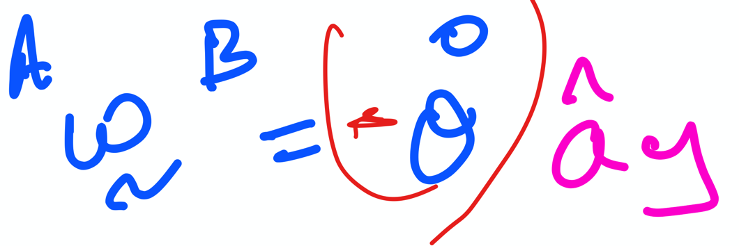
which can both be written in code form below:

A_omega_B_approach1 = - thetadot*A.y
B_omega_C_approach1 = - phidot * (cos(theta)*A.x + sin(theta)*A.z)

Then, we compute the \(^A\omega^C\) by the aforementioned chain rule:

A_omega_C_approach1 = A_omega_B_approach1 + B_omega_C_approach1 # Chain rule
A_omega_C_approach1

\[\displaystyle - \cos{\left(\theta{\left(t \right)} \right)} \frac{d}{d t} \phi{\left(t \right)}\mathbf{\hat{a}_x} - \frac{d}{d t} \theta{\left(t \right)}\mathbf{\hat{a}_y} - \sin{\left(\theta{\left(t \right)} \right)} \frac{d}{d t} \phi{\left(t \right)}\mathbf{\hat{a}_z}\]

Taking the time derivative from \(A\) (i.e., \(\frac{^Ad}{dt}\)) of A_omega_C_approach1 will give us \(^A\alpha^C\), as shown below:

A_alpha_C_approach1 = A_omega_C_approach1.dt(A)
A_alpha_C_approach1

\[\displaystyle (\sin{\left(\theta{\left(t \right)} \right)} \frac{d}{d t} \phi{\left(t \right)} \frac{d}{d t} \theta{\left(t \right)} - \cos{\left(\theta{\left(t \right)} \right)} \frac{d^{2}}{d t^{2}} \phi{\left(t \right)})\mathbf{\hat{a}_x} - \frac{d^{2}}{d t^{2}} \theta{\left(t \right)}\mathbf{\hat{a}_y} + (- \sin{\left(\theta{\left(t \right)} \right)} \frac{d^{2}}{d t^{2}} \phi{\left(t \right)} - \cos{\left(\theta{\left(t \right)} \right)} \frac{d}{d t} \phi{\left(t \right)} \frac{d}{d t} \theta{\left(t \right)})\mathbf{\hat{a}_z}\]

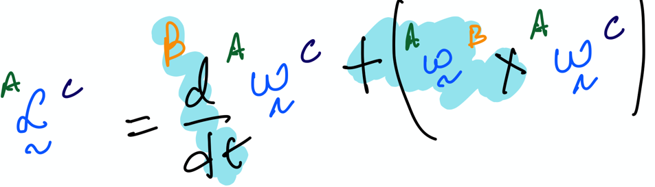
Approach 2: Using key result 2 from lecture notes

Our goal in this subsection is to use an alternate approach to computing \(^A\alpha^C\): by using key rule 2 as shown below:

In the second approach, we again make use of chain rule to compute the \(^A\omega^C\); however, we express all the angular velocities in the B-frame (as done in the notes):

This is implemented below:

A_omega_B_approach2 = - thetadot*B.y
B_omega_C_approach2 = - phidot * B.x
A_omega_C_approach2 = A_omega_B_approach2 + B_omega_C_approach2 # Chain rule again

Then, we implement key result 2 to compute \(^A\alpha^C\) as shown below:

A_alpha_C_approach2 = A_omega_C_approach2.dt(B) + A_omega_B_approach2.cross(A_omega_C_approach2)
A_alpha_C_approach2

\[\displaystyle - \frac{d^{2}}{d t^{2}} \phi{\left(t \right)}\mathbf{\hat{b}_x} - \frac{d^{2}}{d t^{2}} \theta{\left(t \right)}\mathbf{\hat{b}_y} - \frac{d}{d t} \phi{\left(t \right)} \frac{d}{d t} \theta{\left(t \right)}\mathbf{\hat{b}_z}\]