JN5: Practice Activity 4

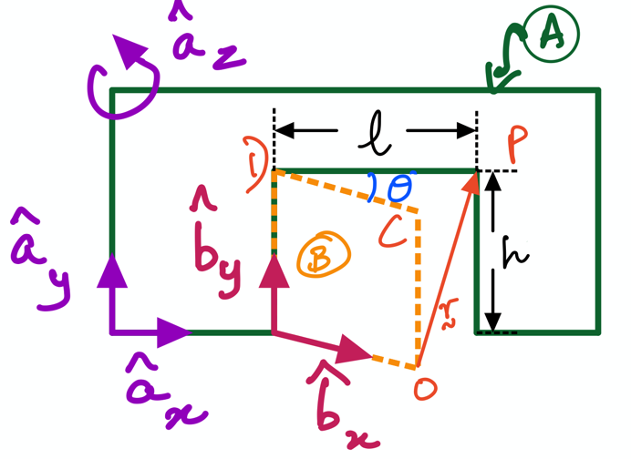
Fig. 8 Motion of a door \(B\) relative to wall \(A\).

This notebook use the door-wall example (see figure above).

To achieve this task, we introduce two important concepts:

1. defining symbols that change with respect to time, using Sympy. We need this because, in the wall-door example above, we know that the angle \(\theta\) changes as a function of time as the door \(B\) swings realtive to wall \(A\).

2. taking time derivatives of vector functions. This is necessary because L3PA3 requires us to compute time derivatives of vector \(\bf r\). Specifically, we are asked to compute \(\frac{^A d}{dt}\bf r\) and \(\frac{^B d}{dt}\bf r\).

Create time-varying scalars using dynamicsymbols

By looking at the figure above humans can quite easily interepret that when the door \(B\) swings realtive to wall \(A\), the angle \(\theta\) between the two objects changes with time. However, computers are not inherently aware of this so we have to be explicit in communicating this to the computer. In sympy, we enforce this by making use of its dynamicsymbols feature to create \(\theta\); this is specifically available within sympy.physics.mechanics.

from sympy.physics.mechanics import dynamicsymbols, init_vprinting
init_vprinting()
theta = dynamicsymbols('theta')

theta

So, what you see from the above output is that \(\theta\) is now very clearly a funciton of time, i.e., \(\theta(t)\). As we will see in the rest of this interactive discussion, time derivatives of those vectors wherein the angle \(\theta\) appears will automatically result in the emergence of \(\dot \theta\); the computer is intelligent enough to know how to treat time-varying scalars once you (the coder) has provided it the basic informaton. Remember that the dot is just short-hand for time derivative of a scalar function, i.e., \(\dot \theta \triangleq \frac{d}{dt}\theta(t)\).

Create constant scalars using symbols

Then, we create the scalars for the length \(l\) and height \(h\) of the door by using the symbols feature; we have already used these in the previous activities. Now, we make it clear that all symbols are treated as constants by sympy. sympy is also intelligent enough to automatically treat them as constants when computing their time derivatives.

from sympy import symbols
l, h = symbols('l h')

l

h

Creating Reference Frames

As taking the derivatives of any vector requires clear information about the reference frame, we create the A and B are reference frames using ReferenceFrame as below:

from sympy.physics.mechanics import ReferenceFrame

A = ReferenceFrame('A')

B = ReferenceFrame('B')

L3PA3

Computing \(\frac{^A d}{dt}\bf r\)

from sympy import sin, cos
r_vec = h*A.y - l * ( cos(theta)*A.x + sin(theta)*A.z ) + l*A.x

r_vec

r_vec.dt(A)

Activity: Computing \(\frac{^B d}{dt}\bf r\)

Please write some code below to compute the \(\frac{^B d}{dt}\bf r\). You may need to insert some additional cells to do so:

Activity: Re-compute \(\frac{^A d}{dt}\bf r\)

Please re-compute the \(\frac{^A d}{dt}\bf r\). Does your answer make sense? Why or why not?