Elliptic Orbits

Prepared by: Noah Leigh, Ilanthiraiyan Sivaganamoorthy, Adriana Lopez, and Angadh Nanjangud

So far, we have studied some general aspects of orbital dynamics without focusing on any specifics shapes of orbits. Here, our main goal is to address this by diving deeper into elliptic orbits. The following sections will support us in learning about elliptic orbits:

1. The Eccentricity Vector

2. The Equation of the Orbit

3. Elliptic Orbits

4. Admissible Orbital Radius

5. Vis-Viva Equation

The Eccentricity Vector

Deriving The Eccentricity Vector

The Eccentricity vector \({\bf e}\) helps us describe the shape of an orbit and its direction. We can find it by taking the cross product of Equation (31) with the specific angular momentum \(\bf h\):

(70)\[\ddot{{\bf r}}\times{\bf h} = - \frac{\mu}{r^3} {\bf r}\times{\bf h}\]

Using the product rule for differentiation, we see that

(71)\[\begin{split}\frac{d}{dt}(\dot{{\bf r}} \times {\bf h}) &= \ddot{{\bf r}} \times {\bf h} + \dot{{\bf r}} \times \dot{{\bf h}} \\ &= \ddot{{\bf r}} \times {\bf h},\end{split}\]

where we note that \(\dot{\bf{h}} = 0\) because \(\bf{h}\) is constant, as shown previously. Therefore, we have shown that the left-hand side of Equation (70) can be written as:

\[\ddot{{\bf r}} \times {\bf h} = \frac{d}{dt}(\dot{{\bf r}} \times {\bf h})\]

Now, we focus on the RHS of Equation (70), which can be written as a vector triple product by substituting \({\bf h}\) as \({\bf r}\cdot\dot{{\bf r}}\):

Note

The general form of the vector triple product \({\bf a}\times ({\bf b}\times{\bf c} )\) is rewritten as \(({\bf c}\cdot{\bf a}){\bf b} - ({\bf b}\cdot{\bf a}){\bf c}\).

(72)\[\begin{split}- \frac{\mu}{r^3} {\bf r}\times{\bf h} &= - \frac{\mu}{r^3} {\bf r} \times\Bigl( {\bf r} \times \dot{\bf r}\Bigr)\\ &=-\frac{\mu}{r^3} \Bigl[ (\dot{{\bf r}}\cdot{\bf r}){\bf r}-({\bf r}\cdot{\bf r})\dot{{\bf r}} \Bigr]\\ &=-\frac{\mu}{r^3}(\dot{r}r{\bf r}-r^2\dot{{\bf r}})\\ &=-\frac{\mu}{r^2}(\dot{r}{\bf r}-r\dot{{\bf r}})\end{split}\]

Now, take a moment to consider the time derivative of the RHS of Equation (70) (and remembering that \(\mu\) is constant) gives the same result as Equation (72)

(73)\[\frac{d}{dt} (\mu \frac{\bf r}{r} ) = - \frac{\mu}{r^2}(\dot{r}{\bf r} - r\dot{\bf r})\]

thus showing that the RHS of Equation (70) is the same as the LHS of Equation (72). That is:

\[\frac{d}{dt}(\dot{{\bf r}} \times {\bf h}) = \frac{d}{dt} (\mu \frac{\bf r}{r} )\]

or that

(74)\[\dot{{\bf r}}\times{\bf h} - \mu\frac{{\bf r}}{r} = constant.\]

We call this entire vectors that results on the LHS of Equation (74) as the eccentricty vector \(\bf e\), which can also be written as:

Note

We have divided throughout Equation (74) by \(\mu\), as this doesn’t really affect things on either side of the equation.

(75)\[{\bf e}=\frac{\dot{{\bf r}}\times{\bf h}}{\mu}-\frac{{\bf r}}{r} \]

Properties of \(\bf e\)

Note

Can you explain why \({\bf e}\) lies in the plane of motion?

1. Again, we remind you that we have derived that \({\bf e}\) is a constant vector. This is implying it is both constant in direction and magnitude. Further, \({\bf e}\) lies in the plane of motion and is fixed. Thus we can arbitrarily choose a direction \(\hat{i}\) t be aligned with \({\bf e}\).

2. Further, \(e = |{\bf e}| \geq 0\), by definition.

The Equation of the Orbit

We derive the equation to the orbit using the eccentricity vector. We begin by taking the dot product of \({\bf e}\) with \({\bf r}\).

Note

recall \({\bf a}\cdot({\bf b}\times{\bf c})=({\bf a}\times{\bf b})\cdot{\bf c}\)

(76)\[\begin{split}{\bf r}\cdot{\bf e} &= \frac{{\bf r}\cdot(\dot{{\bf r}}\times\dot{{\bf h}})}{\mu}-\frac{{\bf r}\cdot{\bf r}}{r}\\ &=\frac{({\bf r}\times\dot{{\bf r}})\cdot{\bf h}}{\mu} - \frac{r^2}{r}\\ &= \frac{h^2}{\mu}-r\end{split}\]

But we also know that \({\bf r}\cdot{\bf e}= r e \cos(\theta)\), where \(\theta\) is the angle between \({\bf r}\) and \({\bf e}\) and is called the true anomaly. Then, we can rewrite Equation (76) as

Note

In some textbooks, \(\theta\) is written by other symbols such as \(\nu\) or \(f\).

\[r e \cos(\theta) = \frac{h^2}{\mu}-r\]

or we can solve for \(r\) as

(77)\[r = \frac{\frac{h^2}{\mu}}{1+ e \cos\left(\theta\right)}\]

This shows that \(r\) is the equation to an ellipse and, in fact, yields Kepler’s 1st Law which states that the orbit of a planet is an ellipse with the sun at one of the two focii.

Actually, \(r\) describes a different conic depending on the eccentricity (a constant that is determined by initial conditions). The eccentricity, \(e=|{\bf e}| \geq 0\), determines the shape of the orbit. Substituting for the different values of \(e\), as given below, into Equation (77) can yield different orbits:

• Circular orbit: \(e = 0 \Rightarrow r = h^2/\mu = const\)

• Elliptic orbit: \(0 < e < 1 \Rightarrow r_{min} < r < r_{max} \)

• Parabolic orbit: \(e = 1 \Rightarrow \frac{1}{2}h^2/\mu \leq r \leq \infty\)

• Hyperbolic orbit: \(e > 1 \Rightarrow \frac{h^2/\mu}{1+e} \leq r \leq \infty \)

Tip

• Operative orbits are always circular or elliptic so as to keep a satellite close to the planet of interest for as long as possible.

• Hyperbolic orbits are essentially maneuvers for interplanetary missions, typically to reduce propellant use by using the gravity of a body to reach another target body (also known as gravity assist maneuver).

Elliptic Orbits

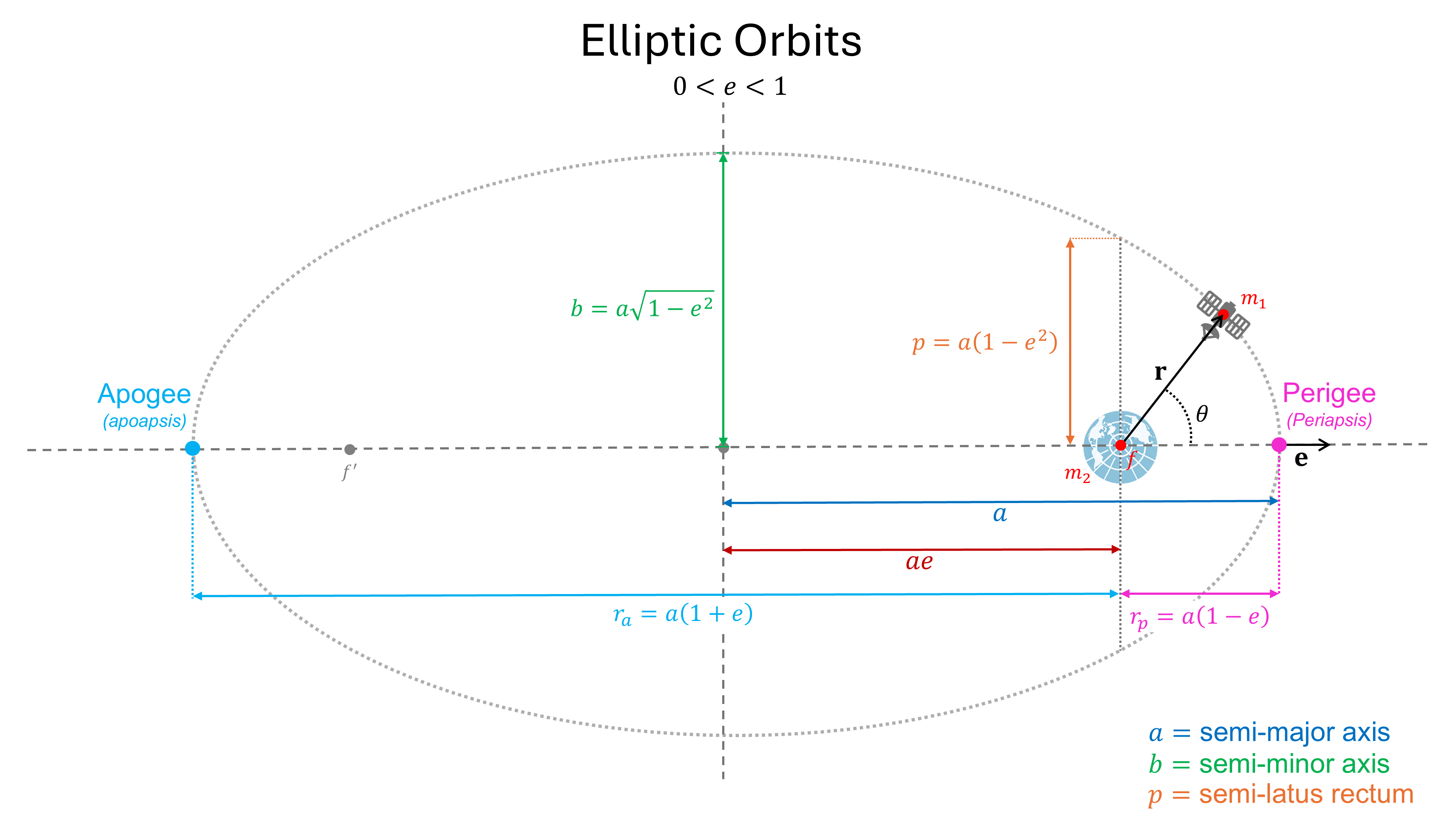
Fig. 6 An ellipse demostrating the different properties of an elliptical orbit, all shown in different colours.

a = semi-major axis
b = semi-minor axis
p = semi-latus rectum
\(\textcolor{#646464}{{\bf e}}\) is aligned with the apsides and point towards the perigee

Key Parameters of Elliptic Orbits

Aside from the equations shown within Fig. 6, we also can determine three other parameters:

1. Semi-latus rectum(\(p\)): This is the distance from the foci (orbitted body) to the orbit measured perpendicular to the semi-major axis. It can be computed from Equation (77) by setting \(\theta = 90^\circ\)

   (78)\[r = \frac{h^2}{\mu} = p\]

   More generally, we can then rewrite Equation (77) using \(p\) as

   (79)\[r = \frac{p}{1 + e \cos\theta} = \frac{a(1 - e^2)}{1 + e \cos\theta}\]

   where,

   (80)\[p = a(1 - e^2)\]

Note

If a satellite is orbiting the moon (mass \(m_2\) in Fig. 6), then we specifically use terms perilune and apolune instead of periapsis and apoapsis. If \(m_2\) is the Earth, then we use the terms perigee and apogee.

2. Periapsis is the value of \(r\) at \(\theta = 0^\circ\) and is denoted \(r_p\). It can be obtained from Equation (79) as

   (81)\[r_p = \frac{p}{1+e}= a(1 - e)\]

3. Apoapsis is the value of \(r\) at \(\theta = 180^\circ\) and is denoted \(r_a\). . It can be obtained from Equation (79) as

   (82)\[r_a = a(1 + e)\]

Determination of the Orbit

Typically you will be given \({\bf r_o}\) and \({\bf v_o}\) and will be asked to compute \({\bf h}\) and \({\bf e}\). The process for doing so is:

1. Compute the semi-latus rectum \(p\) from Equation (78).

2. Compute the semi-major axis, \(a\), using \(a=\frac{p}{1-e^2}\) (shown in Fig. 6).

3. Compute the apsides points (most extreme points in the orbit) using (81) and (82) .

Admissible Orbital Radius

Starting from Equation (69), we can rewrite \(E\) as

(83)\[\begin{split}E &= \frac{1}{2}v^2- \Bigl(\frac{\mu}{r}\Bigr)\\ \Rightarrow E &= \frac{1}{2}{\dot r}^2+\frac{1}{2}r^2 \dot{\theta}^2-\Bigl(\frac{\mu}{r}\Bigr)\\ \Rightarrow E &= \frac{1}{2}{\dot r}^2+\Bigl(\frac{1}{2}\frac{h^2}{r^2}-\frac{\mu}{r}\Bigr)\end{split}\]

Focusing on the terms within the brackets on the RHS of Equation (83), we can define a few terms:

• the entire collection of terms \(\frac{1}{2}\frac{h^2}{r^2}-\frac{\mu}{r}\) is called the effective potential and denoted by \(\phi_{eff}(r)\).

• the first of these terms, \(\frac{1}{2}\frac{h^2}{r^2}\), is known as the potential of the centrifugal force; and

• the second of these terms, \(-\frac{\mu}{r}\), is referred to as the potential of the gravitational force.

Fig. 7 shows a qualitative depiction of the contribution of each of these terms to the effective potential separately and how their sum shapes the effective potential.

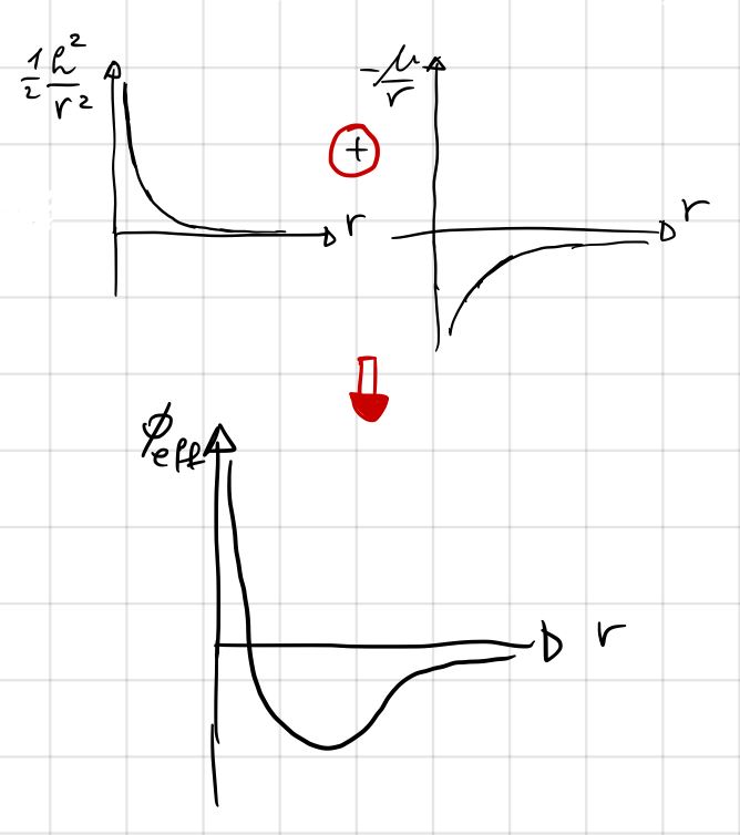
Fig. 7 Qualitative depiction of \(\phi_{eff}(r)\) and its contributions from the two terms in brackets on the RHS of Equation (83).

The effective potential can take positive or negative values over a range of values of \(r\) given its definition.

Now, Equation (83) can be written as

(84)\[E = \frac{1}{2}{\dot r}^2 + \phi_{eff}(r) = constant\]

From this equation, we can infer that:

• the kinetic energy term \(\frac{1}{2}{\dot r}^2 \geq 0\).

• therefore \(E\geq\phi_{eff}(r)\).

Thus motion is only possible for those values of \(r\) such that \(E\geq\phi_{eff}\).

Fig. 8 is a qualitative depiction of the \(\phi_{eff}\) as a function of \(r\):

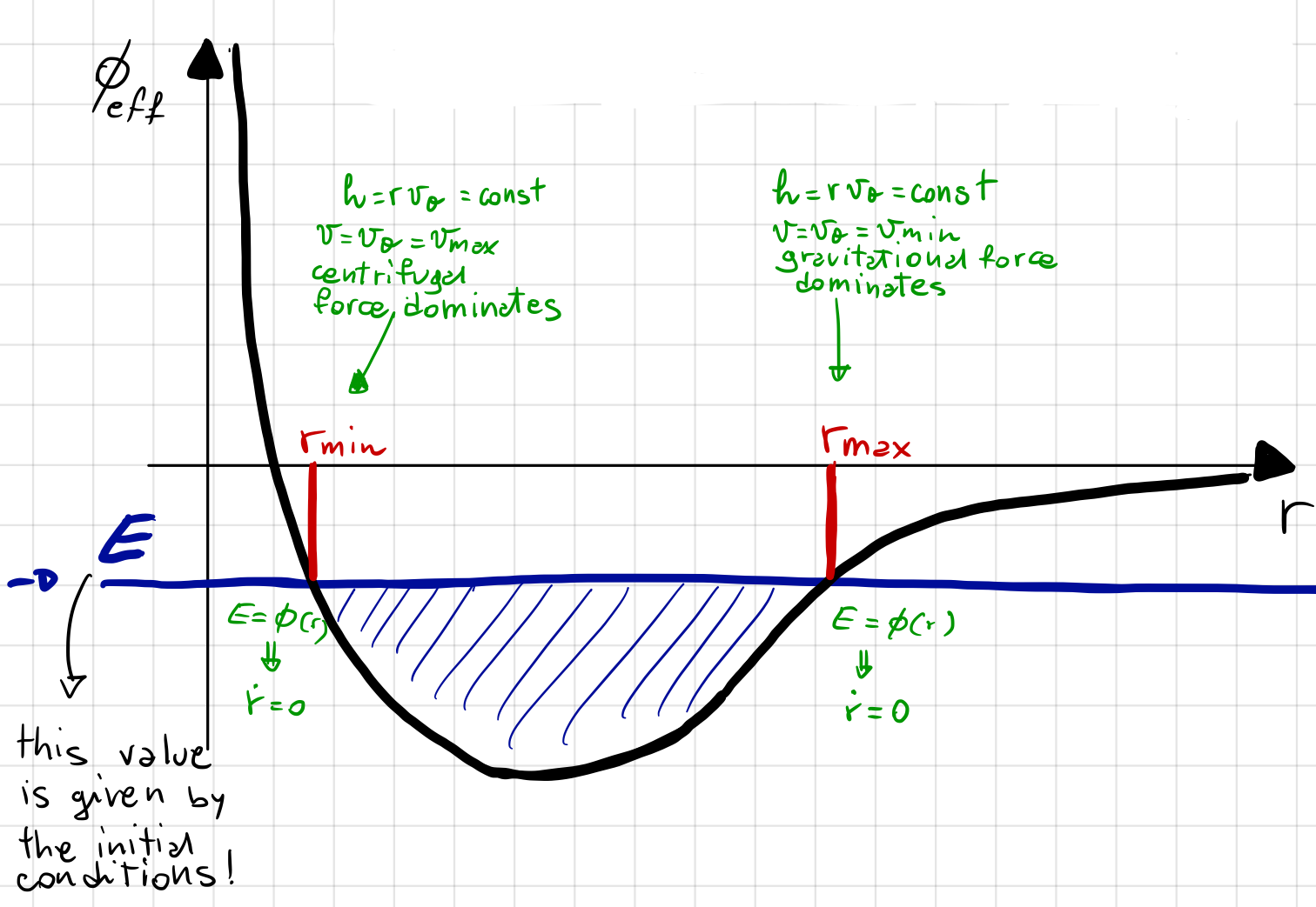
Fig. 8 \(\phi_{eff}\) as a function of \(r\).

This is a more detailed depiction of Fig. 7, which also shows the constant specific energy \(E\) as a blue horizontal line. Indeed, as \(E\) is constant, it can easily be computed from the initial conditions of the system. \(E\) can take on various values, each corresponding to a different orbit:

• When \(E<0\), the motion occurs between \(r_{min}\) and \(r_{max}\) telling us that the motion is bounded. More specifically, it is an elliptical orbit; this condition is shown clearly in Fig. 8.

• When \(E\geq0\) the motion is unbounded; this case is shown in the right side of Fig. 9.

• For \(E=\min{\phi(r)}\), we get the condition that \(r_{min}=r_{max}\) resulting in a circular orbit. This case is shown in the left side ofFig. 9.

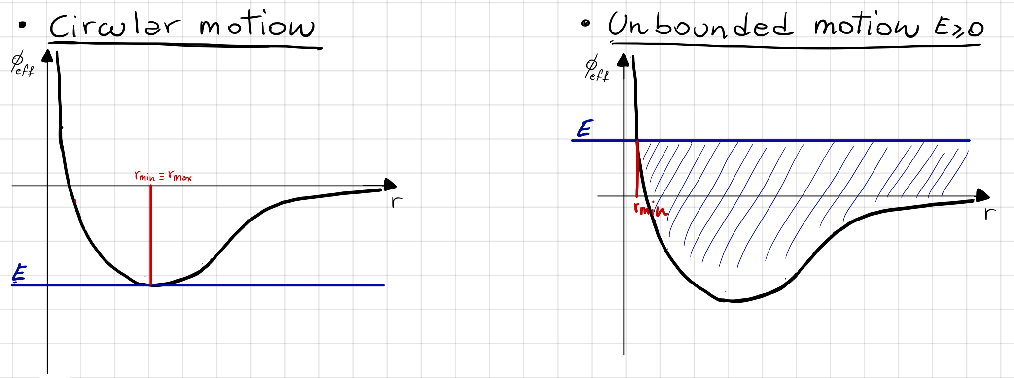
Fig. 9 On the left plot, we see that \(E\) aligns with the minimum value of \(\phi_{eff}\) at \(r_{min}\) and \(r_{max}\). On the right plot, we see that for \(E\geq0\), the motion is unbounded.

Key points

Key takeaways from the discussion so far are that when we are given the initial position \(\bf{r_0}\) and velocity \(\bf{v_0}\) we can compute:

1. Specific angular momentum \(\bf{h}\) as shown below:

(85)\[{\bf h}={\bf h_0}=constant\]

which is orthogonal to the orbital plane. The intial values also tells us that the constant areal velocity is \(\frac{1}{2}r_0^2\dot \theta_0\).

2. Specific orbital energy \(E\) as shown below

(86)\[E_0=\frac{1}{2}v_0^2 - \frac{\mu}{r_0}\]

where \(E_0\) is the specific orbital energy at computed from the initial conditions. If \(E<0\), we have a bounded orbit but if \(E\geq0\) we have unbounded motion.

3. Compute the minimum or maximum values of \(r\) when \(\phi_{eff}=E=E_0\).

Vis-Viva Equation

The Vis-Viva Equation is one of the most useful equations in space mission design as it is used to find the velocity at any given \(r\) when a maneuver is planned.

The total energy of the orbit is the sum of the kinetic energy and the potential energies of the orbit. The sum of the potential energies is the effective potential energy, \(\phi_{eff}\):

Tip

Recall that \({\bf v} = \dot{r}\hat{\bf e}_r + r\dot{\theta}\hat{\bf e}_\theta\). In terms of \(h\), this becomes \({\bf v} = \dot{r}\hat{\bf e}_r + \frac{h}{r}\hat{\bf e}_\theta\). From this, we can now easily compute the magnitude of the velocity as seen in Equation (87).

(87)\[\begin{split}E &= \frac{1}{2} v^2-\frac{\mu}{r}\\ &= \frac{1}{2} \dot{r^2} + \frac{1}{2} \frac{h^2}{r^2} - \frac{\mu}{r}\\ &= \frac{1}{2} \dot{r^2} + \phi_{eff}\end{split}\]

At perigee, \(r_p\), and apogee, \(r_a\), the radial component of velocity in Equation (87), \(\dot r = 0\); at these points, \(E=\phi_{eff}\) which allows us to derive E as a function of the semi-major axis, \(a\).

Tip

We make use of \(r_p\) and \(p\) defined in Equations (82) and (80), respectively.

(88)\[\begin{split}E({r_p})&=\phi_{eff}({r_p})\\ &= \frac{1}{2} \frac{h^2}{r_p^2} - \frac{\mu}{r_p}\\ &= \frac{1}{2} \frac{\mu p}{r_p^2} - \frac{\mu}{r_p}\\ &= -\frac{\mu(1-e)}{2a (1-e)}\\ E&=-\frac{\mu}{2a}\end{split}\]

The specific orbital energy is thus solely a function of \(a\). Orbits with the same semi-major axis have the same specific orbital energy.

The Vis-Viva Equation is obtained by equating Equations (87) and (88) as

Vis Viva Equation

(89)\[\frac{1}{2}v^2 - \frac{\mu}{r}= -\frac{\mu}{2a}\]

Conclusion

• The eccentricity vector is a constant vector in orbital mechanics.

• The orbit equation describes different conic sections based on the magnitude of the eccentricity vector.

• The Vis Viva equation (89) is a crucial tool in mission planning for calculating velocities at various points in an orbit.